The inla.posterior.sample.eval-function

Introduction

This short note add some more explanation to the inla.posterior.sample.eval()-function, as its a constant source of confusing (which is understandable). The purpose of this function is to ease function-evaluations of samples from the fitted model.

Simple example

As often, its easier to work with an example.

n <- 100
x <- rnorm(n)
eta <- 1 + x
y <- rnorm(n, mean = eta, sd = 0.1)
r <- inla(y ~ 1 + x,
    data = data.frame(y,x),
    control.compute = list(config=TRUE))

where the config argument is required. We can now generate samples from the fitted model

samples <- inla.posterior.sample(10000, r)

Here, samples contains the samples, but in long vectors with additional information about where to find what which makes it complicated.

The information available is what is in the output

summary(r)

Time used:
    Pre = 0.354, Running = 0.157, Post = 0.0353, Total = 0.546 
Fixed effects:
             mean    sd 0.025quant 0.5quant 0.975quant  mode kld
(Intercept) 0.990 0.010      0.971    0.990      1.009 0.990   0
x           0.995 0.011      0.974    0.995      1.016 0.995   0

Model hyperparameters:
                                          mean    sd 0.025quant 0.5quant
Precision for the Gaussian observations 108.27 15.31      80.39   107.55
                                        0.975quant   mode
Precision for the Gaussian observations     140.30 106.11

Marginal log-Likelihood:  74.36 
 is computed 
Posterior summaries for the linear predictor and the fitted values are computed
(Posterior marginals needs also 'control.compute=list(return.marginals.predictor=TRUE)')

so its x, (Intercept) and the Precision for the Gaussian observations, plus the linear predictor(s).

The ...eval() function simplifies the evaluation of a function over (joint) samples, by assigning sample-values to each variable. To extract samples of x, which is here the regression coefficient for the covariates $x$ (this is confusing, I know), then we can do

fun1 <- function() return (x)

We can now evaluate fun1 for each sample, using the ...eval()-function, like

eval.fun1 <- inla.posterior.sample.eval(fun1, samples)
str(eval.fun1)

 num [1, 1:10000] 1.006 0.97 0.977 0.998 1.004 ...
 - attr(*, "dimnames")=List of 2
  ..$ : chr "fun[1]"
  ..$ : chr [1:10000] "sample:1" "sample:2" "sample:3" "sample:4" ...

since x is automatically assigned the sample value before fun1 is called. This happens for each sample.

We can compare with the the INLA-output

hist(eval.fun1[1,], prob=TRUE, n=300)
lines(inla.smarginal(r$marginals.fixed$x), lwd=3)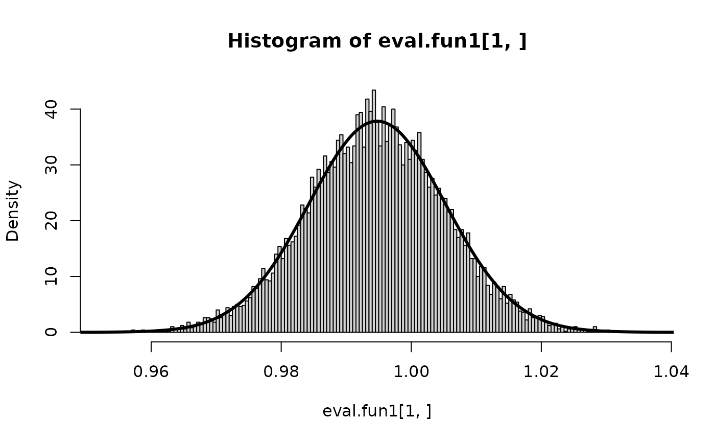

and the results seems to agree.

Also the variable (Intercept) is automatically created, but since this form is awkward to use in R, it is equivalent to Intercept. We can for example sample the linear predictor with

fun2 <- function(x.cov) return (Intercept + x * x.cov)

Here, we need to pass the covariates $x$ (which is not the same as x) separately as a named argument,

eval.fun2 <- inla.posterior.sample.eval(fun2, samples, x.cov = x)

and we plot the regression-line

plot(x, apply(eval.fun2, 1, mean))
abline(a=1, b=1) # this is the true curve

The predictor is also available automatically as Predictor, so

fun3 <- function(x.cov) return (Predictor - (Intercept + x * x.cov))
eval.fun3 <- inla.posterior.sample.eval(fun3, samples, x.cov = x)
summary(eval.fun3[1,])

      Min.    1st Qu.     Median       Mean    3rd Qu.       Max. 
-5.551e-17 -5.551e-17  0.000e+00 -4.940e-19  0.000e+00  5.551e-17

as it should.

Samples of hyper-parameters

It gets a little more involved with the hyper-parameters. In the example above, there is only one, the precision for the observational noise. We can use this to sample new data from the fitted model. Hyper-parameters are automatically assigned values in the vector theta.

fun4 <- function() return (theta)
eval.fun4 <- inla.posterior.sample.eval(fun4, samples)
table(eval.fun4[1, ])


61.6806477523926 72.4386693479479 81.7215542045142 92.1940240166842 
              11               93              541             1452 
 99.911053924203 108.274031887778  116.73423974298 125.855502845737 
            1969             1915             2031             1435 
140.890961882934 157.722647730621 
             505               48

A feature here, is that only the integration points for theta are used, hence samples of theta are discrete with finite number of values. (To only sample the hyper-parameters, please use function inla.hyperpar.sample().) Note that theta, by default, is the hyper-parameters in the user-scale (like precision, correlation, etc). If argument intern=TRUE is used in the inla.posterior.sample()-function, then they will appear in the internal-scale (like log(precision), etc).

We can generate a new dataset from the fitted model, with

samples <- inla.posterior.sample(1, r)
fun4 <- function() {
    n <- length(Predictor)
    return (Predictor + rnorm(n, sd = sqrt(1/theta)))
}
eval.fun4 <- inla.posterior.sample.eval(fun4, samples)
plot(x, eval.fun4[,1])

With more than one hyper-parameter, then theta is vector, and the order of hyper-parameters is the same as is stored in the result-object. The user has to organise this manually. With

r <- inla(y ~ 1 + x,
    family = "sn",
    data = data.frame(y,x),
    control.compute = list(config=TRUE))

then

rownames(r$summary.hyperpar)

[1] "precision for skew-normal observations"
[2] "Skewness for skew-normal observations"

so that theta[1] is the precision while theta[2] is the skewness.

Example: Predictor with and without random effects

Here is an example that pops up from time to time, using the tools above. We are interested in comparing the linear predictor with and without some random effects. The below example is artificial but shows how this works.

First we simulate some data

m <- 100
n <- m^2
## fixed effects
x <- rnorm(n)
xx <- rnorm(n)
## random effects
v <- rnorm(m, sd=0.2)
v.idx <- rep(1:m, each = m)
eta <- 1 + 0.2 * (x + xx) + v
y <- rpois(n, exp(eta))

and then fit the model

r <- inla(y ~ 1 + x + xx + f(v.idx, model = "iid"),
          data = data.frame(y, x, xx, v.idx),
          family = "poisson",
          control.compute = list(config = TRUE))
samples <- inla.posterior.sample(10000, r)

Now we want to compare the linear predictor with and without the f(v.idx, model = "iid") term. The easy way out, is to use the predictor and then subtract the iid-term, instead of building it up manually.

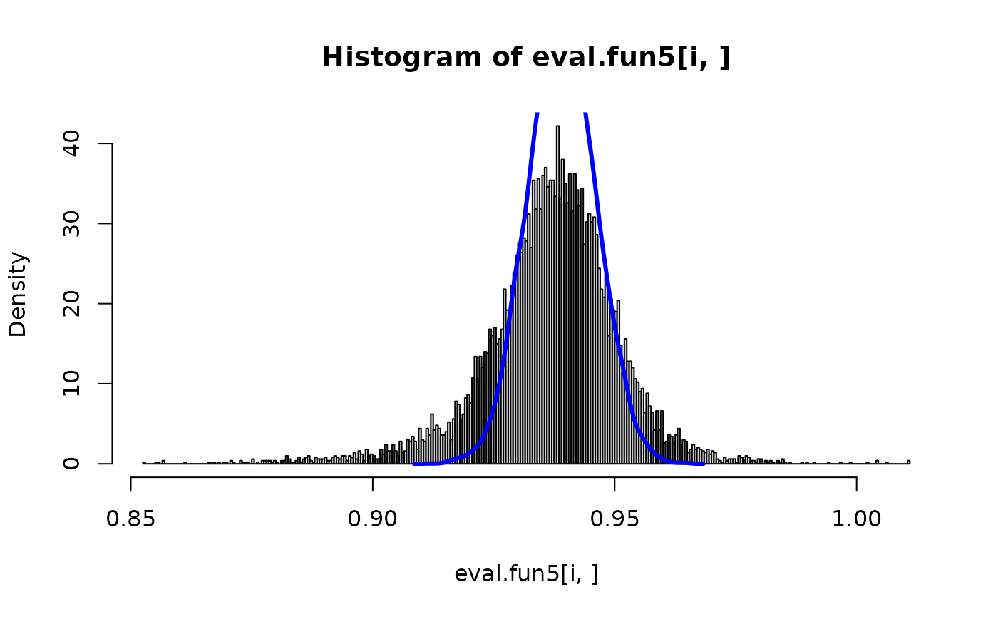
fun5 <- function(v.index) {
    return (c(Predictor, Predictor - v.idx[v.index]))
}
eval.fun5 <- inla.posterior.sample.eval(fun5, samples, v.index=v.idx)

And we can compare with and without for some components

i <- 2
hist(eval.fun5[i,], prob=TRUE, n=300)
lines(density(eval.fun5[n + i,]), col="blue", lwd=3)

Predictor $A$ -matrix (experimental-mode only)

For some models, especially models using the SPDE, then a projector matrix is used, so we need the A-matrix for the predictor. Often this looks like

r <- inla(...., control.predictor = list(A=inla.stack.A(...)))

For these models, then the observations depend on $\eta^*$ , where $\eta^* = A \eta$ , and $\eta$ is defined with the formula. In these cases, then Predictor is $\eta$ and APredictor is $\eta^*$ . Moreover, the $A$ matrix is available as pA in the ...eval()-function.

Here is the same example above, with a random $A$ -matrix showing how to use this.

n <- 100
m <- 25
## fixed effects
x <- rnorm(n)
xx <- rnorm(n)
## random effects
v <- rnorm(m, sd=0.2)
v.idx <- rep(1:m, each = n %/% m)
eta <- 1 + 0.2 * (x + xx) + v
A <- matrix(rnorm(n^2, sd=sqrt(1/n)), n, n)
eta.star <- A %*% eta
y <- rpois(n, exp(eta.star))

r <- inla(y ~ 1 + x + xx + f(v.idx, model = "iid"),
          data = data.frame(y, x, xx, v.idx),
          family = "poisson",
          inla.mode = "experimental",
          control.predictor = list(A=A),
          control.compute = list(config = TRUE))
samples <- inla.posterior.sample(10000, r)

We will compare the same change, with and without the iid-term.

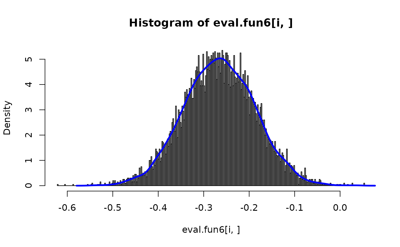
fun6 <- function(v.index) {
    return (c(APredictor, as.numeric(pA %*% (Predictor - v.idx[v.index]))))
}
eval.fun6 <- inla.posterior.sample.eval(fun6, samples, v.index=v.idx)
i <- 2
hist(eval.fun6[i,], prob=TRUE, n=300)
lines(density(eval.fun6[n + i,]), col="blue", lwd=3)

Haavard Rue

KAUST, Aug 2022

Introduction

Simple example

Samples of hyper-parameters

Example: Predictor with and without random effects

Predictor $A$ -matrix (experimental-mode only)

The inla.posterior.sample.eval-function

Haavard Rue

KAUST, Aug 2022

Introduction

Simple example

Samples of hyper-parameters

Example: Predictor with and without random effects

Predictor AA-matrix (experimental-mode only)

Predictor $A$ -matrix (experimental-mode only)