Spatially Varying Coefficient Models with R-INLA
Timothy D. Meehan (tmeeha@gmail.com), Elias T. Krainski, Finn Lindgren, and Håvard Rue
Generated on 2026-04-04
svc.RmdNote: See https://inlabru-org.github.io/inlabru/articles/svc.html
for an updated version of this vignette that avoids manual handling of
mesh indices, mapping matrices, and data stacks, by using the
inlabru interface instead of plain INLA.
Introduction
Spatially varying coefficient models (SVCs, Gelfand et al. 2003) are
often used to model data when relationships between dependent and
independent variables are not uniform across space, a common situation
when exploring phenomena across large spatial extents (Finley 2011).
Meehan et al. (2019) described an SVC model to evaluate continent-scaled
variation in bird abundance trends. The SVC model used in that analysis
employed discrete aerial units (100 km grid cells), with spatial
structure described by neighborhood matrices and spatial relationships
described by an intrinsic conditional autoregressive model (Besag 1974).
The online supplement for the paper included code for building the model
using the R-INLA package (Rue et al. 2009) for the
R statistical programming language (R Core Team 2021). Both
the manuscript and code can be accessed at https://github.com/tmeeha/inlaSVCBC.
In this vignette, we will describe how to build an SVC model similar
to that described in Meehan et al. (2019), but within a continuous-space
framework. This model will be computed using the stochastic partial
differential equation (SPDE) approach of Lindgren et al. (2011, 2022),
implemented in the R-INLA package for R. The
SPDE approach employs a computationally efficient approximation of a
Gaussian random field with parameters directly comparable to those of a
Matérn covariance function. The benefits of a continuous-space versus a
discrete-space SVC include the potential for finer resolution estimation
and prediction, a better understanding of the range of spatial
correlation, and a reduction in boundary effects associated with
discrete-space analyses.
We build the model using a subset of the data described in Meehan et al. (2019). Specifically, we use counts of American Robin (Turdus migratorius) from south central North America collected between 1987 and 2016 during the Audubon Christmas Bird Count (CBC). The overall goal of the analysis is to produce spatially explicit estimates of annual relative abundance as well as long-term relative abundance trends for robins that account for spatial and temporal variation in count effort.
Model
The model used to analyze these data assumes that counts come from a negative binomial distribution with an expected count and dispersion parameter. The expected count has a log-linear predictor:
where the natural log of expected count, , at site during year , is modeled with a zero-centered, normally distributed intercept per site, , a spatially varying intercept, , a spatially varying effect of the log of count effort in hours, , and a spatially varying linear effect of year, . The spatially structured effects are modeled as Gaussian random fields with Matérn covariance functions with range and variance parameters.
Model parameters , , and are analogous to those in Meehan et al. (2019). For example, is included to account for site-level differences in counts, possibly due to habitat availability or observer experience. can be interpreted as an effort-corrected abundance index at year zero. is the exponent for a power-law effort-correction function. And is the long-term temporal trend at a given site.
Environment
To get started with data analysis, we set up the environment, by loading some packages, and setting some options.
# libraries
library(maps)
library(ggplot2)
library(sf)
library(terra)
library(tidyterra) # raster plotting
library(tidyr)
library(scales)
library(inlabru)
library(INLA)
library(dplyr)
# Note: the 'splancs' package also needs to be installed,
# but doesn't need to be loaded

# set option
select <- dplyr::select
options(scipen = 99999)
options(max.print = 99999)
options(stringsAsFactors = FALSE)
Next we define a coordinate reference system (CRS) for spatial analysis and create a base map for later use. The CRS uses the USA Contiguous Albers Equal-Area Conic projection, and is identified by the EPSG code 6703. We modify the CRS slightly to have units of kilometers, so that distances between widespread count sites are not especially large numbers (Krainski et al. 2018).
# define a crs
epsg6703km <- paste(
  "+proj=aea +lat_0=23 +lon_0=-96 +lat_1=29.5",
  "+lat_2=45.5 +x_0=0 +y_0=0 +datum=NAD83",
  "+units=km +no_defs"
)

# make a base map
states <- maps::map("state", plot = FALSE, fill = TRUE) %>%
  sf::st_as_sf() %>%
  filter(ID %in% c(
    "texas", "oklahoma", "kansas", "missouri",
    "arkansas", "louisiana"
  )) %>%
  sf::st_make_valid() %>%
  sf::st_transform(epsg6703km) %>%
  sf::st_make_valid()
Import data
Next we import some bird count data from the GitHub repository associated with Meehan et al. (2019), and turn the data set into spatially referenced points. We use a subset of the data (30 years, 6 US states) for this analysis to reduce computing time (~ 1 min). Note that site selection and zero filling, important components of trend analyses, have already been conducted and this is the resulting data set.
# get data
## download_dat <- read.csv(paste0(
##      "https://raw.github.com/tmeeha/inlaSVCBC",
##      "/master/code/modeling_data.csv"))
download_dat <- read.csv("data/modeling_data.csv.gz")

# select subset
count_dat <- download_dat %>%
  select(
    circle, bcr, state, year, std_yr, count, log_hrs,
    lon, lat, obs
  ) %>%
  mutate(year = year + 1899) %>%
  filter(
    state %in% c(
      "TEXAS", "OKLAHOMA", "KANSAS", "MISSOURI",
      "ARKANSAS", "LOUISIANA"
    ),
    year >= 1987
  )
After loading the data, we filter out observation sites with less
than 20 years of data, add index variables to uniquely index site and
year information, and transform the coordinates to the
epsg6703km CRS:
count_dat <- count_dat %>%
  mutate(site_idx = as.numeric(factor(paste(circle, lon, lat)))) %>%
  group_by(site_idx) %>%
  mutate(n_years = n()) %>%
  filter(n_years >= 20) %>%
  ungroup() %>%
  mutate(
    std_yr = year - max(year),
    obs = seq_len(nrow(.)),
    site_idx = as.numeric(factor(paste(circle, lon, lat))),
    year_idx = as.numeric(factor(year)),
    site_year_idx = as.numeric(factor(paste(circle, lon, lat, year)))
  ) %>%
  st_as_sf(coords = c("lon", "lat"), crs = 4326, remove = FALSE) %>%
  st_transform(epsg6703km) %>%
  mutate(
    easting = st_coordinates(.)[, 1],
    northing = st_coordinates(.)[, 2]
  ) %>%
  arrange(circle, year)
A rough view of changes in robin relative abundance, which does not account for variation in count effort, can be seen by plotting raw counts per site and year.
# map it
ggplot() +
  geom_sf(
    data = count_dat %>% filter(year_idx %in% seq(1, 30, 3)),
    aes(col = log(count + 1))
  ) +
  geom_sf(data = states, fill = NA) +
  coord_sf(datum = NA) +
  facet_wrap(~year) +
  scale_color_distiller(palette = "Spectral") +
  theme_bw()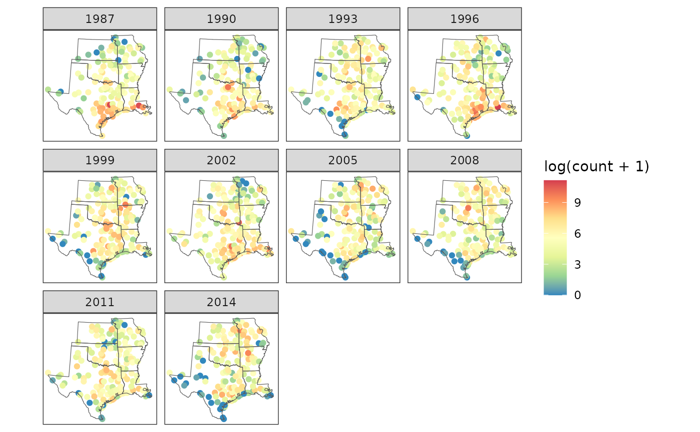
Make spatial data
Next we use the count data to make a map of distinct count sites and save the coordinates of the sites, unique and across all years, for later spatial modeling and plotting.
# make a set of distinct study sites for mapping
site_map <- count_dat %>%
  select(circle, easting, northing) %>%
  distinct() %>%
  select(circle, easting, northing)

# save coordinates as matrices for later
unique_coords <- count_dat %>%
  select(circle, easting, northing) %>%
  distinct() %>%
  select(easting, northing) %>%
  st_drop_geometry() %>%
  as.matrix()
all_coords <- as.matrix(st_coordinates(count_dat))
SPDE components
Computing a continuous-space model with R-INLA using the
SPDE approach requires construction of four distinct sets of data and
model objects (Blangiardo and Cameletti 2015, Krainski et al. 2018).
First, we create a modeling mesh, which is used to
provide a piecewise linear representation of the continuous spatial
surface, based on a triangulation of the modeled region. Here, the same
mesh will get reused for each of the spatial and spatio-temporal terms
in the model. Second, we construct an SPDE model object
that specifies properties of the spatial model. Again, we will use the
same SPDE object for each of the spatial terms in the model. Third, we
create named index sets that identify data locations
and mesh nodes for use in model construction, computation, and output
extraction. Note that a separate set of indices needs to be constructed
for each spatial term in the model. Fourth, we construct
projector matrices or A matrices that
create formulaic mappings between the observed data locations and the
mesh nodes. Again, note that a separate set of projector matrices needs
to be constructed for each spatial term in the model. The four
corresponding functions for these steps are:
fmesher::fm_mesh_2d(), inla.spde2.pcmatern(),
inla.spde.make.index(), and
inla.spde.make.A().
Modeling mesh
There are various things to consider when constructing a mesh (Lindgren and Rue 2015, Blangiardo and Cameletti 2015, Krainski et al. 2018, Bakka et al. 2018). In constructing one, we balance a trade-off between capturing fine-scaled features of the Gaussian random field and computing times. Here, we create a non-convex hull around the count sites, and then build a triangular mesh by specifying minimum and maximum edge lengths within and slightly outside the hull.
# make a hull and mesh for spatial model
hull <- fm_nonconvex_hull(
  count_dat,
  convex = 200,
  concave = 350
)
mesh <- fm_mesh_2d(
  boundary = hull, max.edge = c(100, 600), # km inside and outside
  cutoff = 50, offset = c(100, 300),
  crs = fm_crs(count_dat)
) # cutoff is min edge
# plot it
ggplot() +
  gg(data = mesh) +
  geom_sf(data = site_map, col = "darkgreen", size = 1) +
  geom_sf(data = states, fill = NA) +
  theme_bw() +
  labs(x = "", y = "")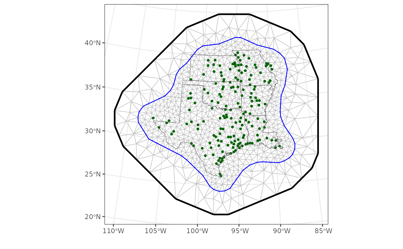
SPDE model object
Next we create an SPDE object to define the model smoothness, with
prior distributions for the variance and range parameters, and the mesh.
Here we assume a Gaussian random field characterized with a Matérn
covariance function with penalized complexity priors (Simpson et
al. 2017) for the practical range (distance where spatial correlation
approaches 0.1) and variation explained by the function (Fuglstad et
al. 2019). The prior for the spatial range is set such that the
probability of a range exceeding 500 km is 0.5. The prior for the
variance explained by the spatial effect is set such that the
probability of a standard deviation exceeding 1 is 0.5 (Krainski et
al. 2018). If one wants to constrain this kind of spatial effect to
integrate to zero, constr=TRUE should be added at this
stage.
# make spde
spde <- inla.spde2.pcmatern(
  mesh = mesh,
  prior.range = c(500, 0.5),
  prior.sigma = c(1, 0.5)
)
Index sets
Next we create index sets for the spatial terms in the model. Note
that the tag names applied to the index sets in this step
will be used in the model formula statement below. The index vectors for
the spatial terms are essentially vectors of integers going from 1 to
the number of nodes on the mesh.
# make index sets
alpha_idx <- inla.spde.make.index(name = "alpha", n.spde = mesh$n)
eps_idx <- inla.spde.make.index(name = "eps", n.spde = mesh$n)
tau_idx <- inla.spde.make.index(name = "tau", n.spde = mesh$n)
Projector matrices
Next we create projector matrices for the spatial terms in the model.
Note that this is the step where SVCs are specified. In our model,
is a spatially varying effect of the log of count effort. The SVC effort
effect is specified using the weights argument to
inla.spde.make.A() function. Similarly,
is a spatially varying effect of year, so standardized year (with 1987 =
0) is also specified in the weights argument.
is also an SVC, but it is a spatially varying intercept. For intercepts
it is not necessary to specify a constant weight of 1 when making a
projector matrix. The only model component ignored here is
,
because it is not spatially structured and not modeled on the mesh. Note
that the current use of the term ‘weights’ is different from that often
encountered when defining mixed effect models in R. Here it
is used to define covariate values, as opposed to importance values in
other contexts.
# make projector matrices
A_alpha <- inla.spde.make.A(mesh = mesh, loc = count_dat)
A_eps <- inla.spde.make.A(
  mesh = mesh, loc = count_dat,
  weights = count_dat$log_hrs
) # note weights argument
A_tau <- inla.spde.make.A(
  mesh = mesh, loc = count_dat,
  weights = count_dat$std_yr
) # note weights argument
Data stack for model fitting
With the SPDE method, there are several data structures that need to
be bundled and used for analysis of the spatial model. There is the
observed response at the count sites, the covariate values at the count
sites, and the indices and mapping of those data to the modeling mesh.
All of this information gets bundled into a data stack for model
analysis using the inla.stack() function. This function is
a very flexible and can be difficult to understand at first. See
Blandgiardo and Cameletti (2015) and Gomez-Rubio (2020) for practical
information on how to use it.
The first argument to the function, shown below, is the
tag name for the stack. In this case we are including
observed data for model estimation, so we name the stack ‘obs’. The next
argument, data, specifies the response variable. Here we
have a single response variable called ‘count’. We tell the stacking
function that observed counts reside in the ‘count_dat’ data set. The
next argument, effects, is used to specify the model
predictors. These are defined using the observed data for non-spatial
predictors, and using the named index sets for the spatial predictors.
The last argument, A, asks for a list of projector matrices
or A matrices for the predictor variables. We did not need to make a
projector for
,
because it is not defined as a spatial parameter. Nevertheless, we add a
value of 1 because it is the value that will be multiplied by the effect
during model computations and serves as a way for the stacking function
to match the number of A matrices with the number of effects – if there
are 4 effects, then there must be four entries for A. Note
that if there were more than one non-spatial predictor in the model,
whether a grouped random intercept or a global fixed effect, then each
one would be given its own value of 1 during this step. And note that
the order of the A matrices must match the order of the effects.
# stack observed data
stack_fit <- inla.stack(
  tag = "obs",
  data = list(count = as.vector(count_dat$count)), # response from data frame
  effects = list(data.frame(
    intercept = 1,
    kappa = count_dat$site_idx
  ), # predictors from data frame
  alpha = alpha_idx, # or index sets if spatial
  eps = eps_idx,
  tau = tau_idx
  ),
  A = list(
    1, # a value of 1 is given for non-spatial terms
    A_alpha,
    A_eps,
    A_tau
  )
)
Model formula
The last required input for the analysis is the model formula, which includes information on the prior for explained variation for the unstructured random intercept. We define the prior for as a penalized complexity prior (Simpson et al. 2017), set such that the probability of the standard deviation associated with the random effect exceeding 1 is 0.01.
Notice that if one wants to constrain a spatial spde effect to
integrate to zero, it should be added constr=TRUE in the
SPDE model definition rather than in the f() terms. As we
want to constrain
and it is a non-spatial term we can use constr=TRUE in its
corresponding f() below, which imposes a sum-to-zero
constraint.
The model described above is translated to R-INLA
modeling syntax as:
# formula
svc_form <- count ~ -1 +
  f(kappa, model = "iid", constr = TRUE, hyper = list(prec = pc_prec)) +
  f(alpha, model = spde) +
  f(eps, model = spde) +
  f(tau, model = spde)
Here, we define the response as count, remove the
automatic global intercept with a -1, and then specify the
other terms in the model with f() statements. The first
f() statement defines
,
the site effect, as a normally distributed (model="iid"),
zero-centered (constr=TRUE), deviation from
.
The name ‘kappa’ given in the f() argument is associated
with the effect ‘kappa’ defined in the estimation stack. The second
f() statement defines
as a spatially varying intercept with spatial structure described by the
SPDE object called ‘spde’. The third f() statement defines
as an SVC for the effect of count effort, with spatial structure also
described by the SPDE object. The weights for this spatially structured
random slope were specified during construction of the projector A
matrix, A_eps. The fourth f() statement
defines
as an SVC for the year effect, with spatial structure described in the
SPDE object. Again, the weights for this spatially structured random
slope were specified during construction of the projector A matrix,
A_tau. Again, note that the current use of the term
‘weights’ is different from that often encountered when defining mixed
effect models in R. Here it is used to define covariate
values, as opposed to importance values in other contexts.
Run model
We estimate the model with a call to inla(). First we
set the option to use the (new) experimental way to do internal
computations, see Van Niekerk et. al. (2022), for the sake of computing
speed and better numerics. In the call to inla(), we give
the model formula, specify the negative binomial distribution for the
counts, define the estimation data, and describe the location of the
projector A matrix. Note that we are not generating predictions
(compute=F). Nevertheless, the
control.preditor argument still needs to be included so the
software knows how to find the A matrices. Then we ask
inla() to compute WAIC and CPO to evaluate model fit, and
to save the information necessary for posterior sampling
(config=T). For computing speed, we choose to use the
adaptive integration strategy and Empirical Bayes estimation. The
inla() run for this model takes about 1 minutes on a
standard laptop computer. Another option is to use the Variational Bayes
approximation as detailed in Van Niekerk and Rue (2021) and Van Niekerk
et. al. (2022).
res <- inla(svc_form,
  family = "nbinomial",
  data = inla.stack.data(stack_fit), # stack the stack
  control.predictor = list(
    A = inla.stack.A(stack_fit),
    compute = FALSE
  ), # must define A
  control.compute = list(waic = TRUE, cpo = TRUE, config = TRUE),
  control.inla = list(strategy = "adaptive", int.strategy = "eb"),
  verbose = FALSE
)
Model summaries
Once computation is complete, we look at the initial results to see how things went. First we check the posterior means for the hyperparameters of the model, mainly the variance components and the spatial ranges of the spatially structured parameters.
# view results
res$summary.hyperpar[-1, c(1, 2)]
## mean sd
## Precision for kappa 2.27817836 0.45827318
## Range for alpha 960.00671132 323.62442997
## Stdev for alpha 1.97445598 0.40639278
## Range for eps 7597.09953846 7624.42058303
## Stdev for eps 0.57044025 0.52591014
## Range for tau 853.86663148 398.90099974
## Stdev for tau 0.06440513 0.01356288Next we examine some summaries of the random effect estimates, starting with , which is effort-corrected relative abundance at year = 0 (1987), given 1 hour of count effort (i.e., log[1]=0).
##     Min.  1st Qu.   Median     Mean  3rd Qu.     Max.
##  0.05909  1.16663  3.41859  7.00562  8.72709 55.00893
Note that to avoid issues due to , we use the posterior median instead of the posterior mean.
The summary for shows variation in the exponent for the effort correction function across space.
summary(res$summary.random$eps$mean) # epsilon## Min. 1st Qu. Median Mean 3rd Qu. Max.
## 0.7883 0.8911 0.9765 0.9639 1.0382 1.1138The summary shows how long-term, log-linear trends of robin relative abundance have varied across space, from annual decreases of around 10% to annual increases of around 10%.
##     Min.  1st Qu.   Median     Mean  3rd Qu.     Max.
## -12.7646  -4.9014  -1.5118  -0.9993   2.7372  10.8899
SVC maps
Next we create maps of , , and to inspect the spatial structure of these parameter estimates. We start by creating a 25-km mapping grid, and then projecting this mapping grid to the modeling mesh.
# get easting and northing limits
bbox <- fm_bbox(hull[[1]])
grd_dims <- round(c(x = diff(bbox[[1]]), y = diff(bbox[[2]])) / 25)

# make mesh projector to get model summaries from the mesh to the mapping grid
mesh_proj <- fm_evaluator(
  mesh,
  xlim = bbox[[1]], ylim = bbox[[2]], dims = grd_dims
)
Then we populate the mapping grids with parameter estimates (posterior median and range95), turn them into a raster stack, and mask the raster stack to the study area.
# pull data
kappa <- data.frame(
  median = exp(res$summary.random$kappa$"0.5quant"),
  range95 = exp(res$summary.random$kappa$"0.975quant") -
    exp(res$summary.random$kappa$"0.025quant")
)
alph <- data.frame(
  median = exp(res$summary.random$alpha$"0.5quant"),
  range95 = exp(res$summary.random$alpha$"0.975quant") -
    exp(res$summary.random$alpha$"0.025quant")
)
epsi <- data.frame(
  median = res$summary.random$eps$"0.5quant",
  range95 = (res$summary.random$eps$"0.975quant" -
    res$summary.random$eps$"0.025quant")
)
taus <- data.frame(
  median = (exp(res$summary.random$tau$"0.5quant") - 1) * 100,
  range95 = (exp(res$summary.random$tau$"0.975quant") -
    exp(res$summary.random$tau$"0.025quant")) * 100
)

# loop to get estimates on a mapping grid
pred_grids <- lapply(
  list(alpha = alph, epsilon = epsi, tau = taus),
  function(x) as.matrix(fm_evaluate(mesh_proj, x))
)
# make a terra raster stack with the posterior median and range95
out_stk <- rast()
for (j in 1:3) {
  mean_j <- cbind(expand.grid(x = mesh_proj$x, y = mesh_proj$y),
    Z = c(matrix(pred_grids[[j]][, 1], grd_dims[1]))
  )
  mean_j <- rast(mean_j, crs = epsg6703km)
  range95_j <- cbind(expand.grid(X = mesh_proj$x, Y = mesh_proj$y),
    Z = c(matrix(pred_grids[[j]][, 2], grd_dims[1]))
  )
  range95_j <- rast(range95_j, crs = epsg6703km)
  out_j <- c(mean_j, range95_j)
  terra::add(out_stk) <- out_j
}
names(out_stk) <- c(
  "alpha_median", "alpha_range95", "epsilon_median",
  "epsilon_range95", "tau_median", "tau_range95"
)
out_stk <- terra::mask(
  out_stk,
  terra::vect(sf::st_union(states)),
  updatevalue = NA,
  touches = FALSE
)
Finally, we plot the SVCs with the following code. We plot the posterior median and 95% uncertainty width (“range95”) for , , , and .
make_plot_field <- function(data_stk, scale_label) {
  ggplot(states) +
    geom_sf(fill = NA) +
    coord_sf(datum = NA) +
    geom_spatraster(data = data_stk) +
    labs(x = "", y = "") +
    scale_fill_distiller(
      scale_label,
      palette = "Spectral",
      na.value = "transparent"
    ) +
    theme_bw() +
    geom_sf(fill = NA)
}
make_plot_site <- function(data, scale_label) {
  ggplot(states) +
    geom_sf() +
    coord_sf(datum = NA) +
    geom_sf(data = data, size = 1, mapping = aes(colour = value)) +
    scale_colour_distiller(scale_label, palette = "Spectral") +
    labs(x = "", y = "") +
    theme_bw() +
    geom_sf(fill = NA)
}

# medians
# fields alpha_s, epsilon_s, tau_s
pa <- make_plot_field(
  data_stk = out_stk[["alpha_median"]],
  scale_label = "posterior\nmedian\nexp(alpha_s)"
)
pe <- make_plot_field(
  data_stk = out_stk[["epsilon_median"]],
  scale_label = "posterior\nmedian\nepsilon_s"
)
pt <- make_plot_field(
  data_stk = out_stk[["tau_median"]],
  scale_label = "posterior\nmedian\n100(exp(tau_s)-1)"
)
# sites kappa_s
ps <- make_plot_site(
  data = cbind(site_map, data.frame(value = kappa$median)),
  scale_label = "posterior\nmedian\nexp(kappa_s)"
)
# range95
# fields alpha_s, epsilon_s, tau_s
pa_range95 <- make_plot_field(
  data_stk = out_stk[["alpha_range95"]],
  scale_label = "posterior\nrange95\nexp(alpha_s)"
)
pe_range95 <- make_plot_field(
  data_stk = out_stk[["epsilon_range95"]],
  scale_label = "posterior\nrange95\nepsilon_s"
)
pt_range95 <- make_plot_field(
  data_stk = out_stk[["tau_range95"]],
  scale_label = "posterior\nrange95\n100(exp(tau_s)-1)"
)
# sites kappa_s
ps_range95 <- make_plot_site(
  data = cbind(site_map, data.frame(value = kappa$range95)),
  scale_label = "posterior\nrange95\nexp(kappa_s)"
)
# plot together
multiplot(ps, pa, pe, pt, cols = 2)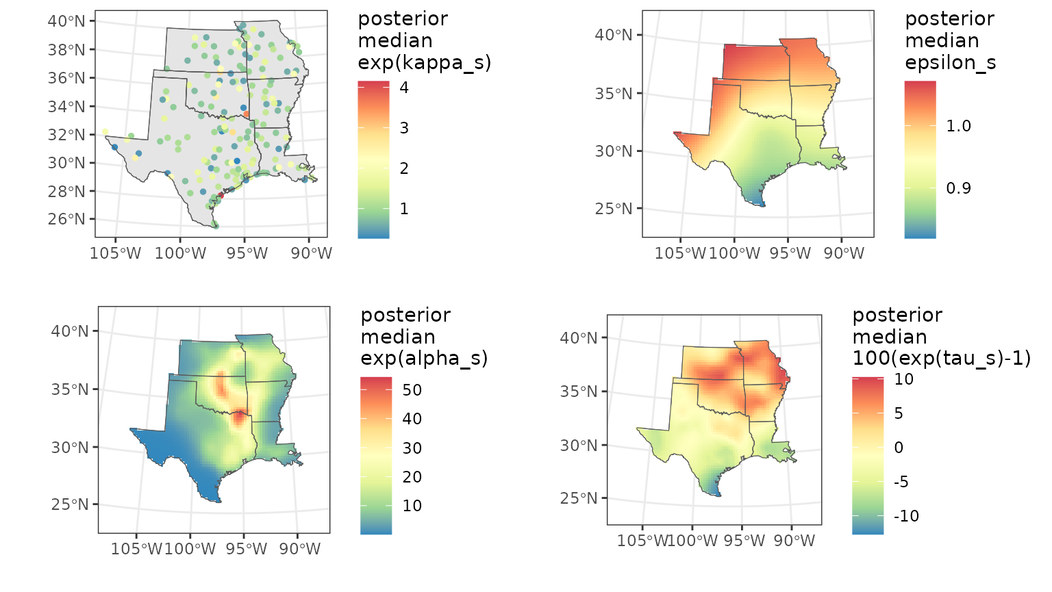 The map for the posterior mean of
shows that robins have decreased in the southern part of the study area
and increased in the northern part. This demonstrates how the wintering
range of robins is shifting northward as winters become warmer due to
climate change.
The map for the posterior mean of
shows that robins have decreased in the southern part of the study area
and increased in the northern part. This demonstrates how the wintering
range of robins is shifting northward as winters become warmer due to
climate change.
# plot together
multiplot(ps_range95, pa_range95, pe_range95, pt_range95, cols = 2)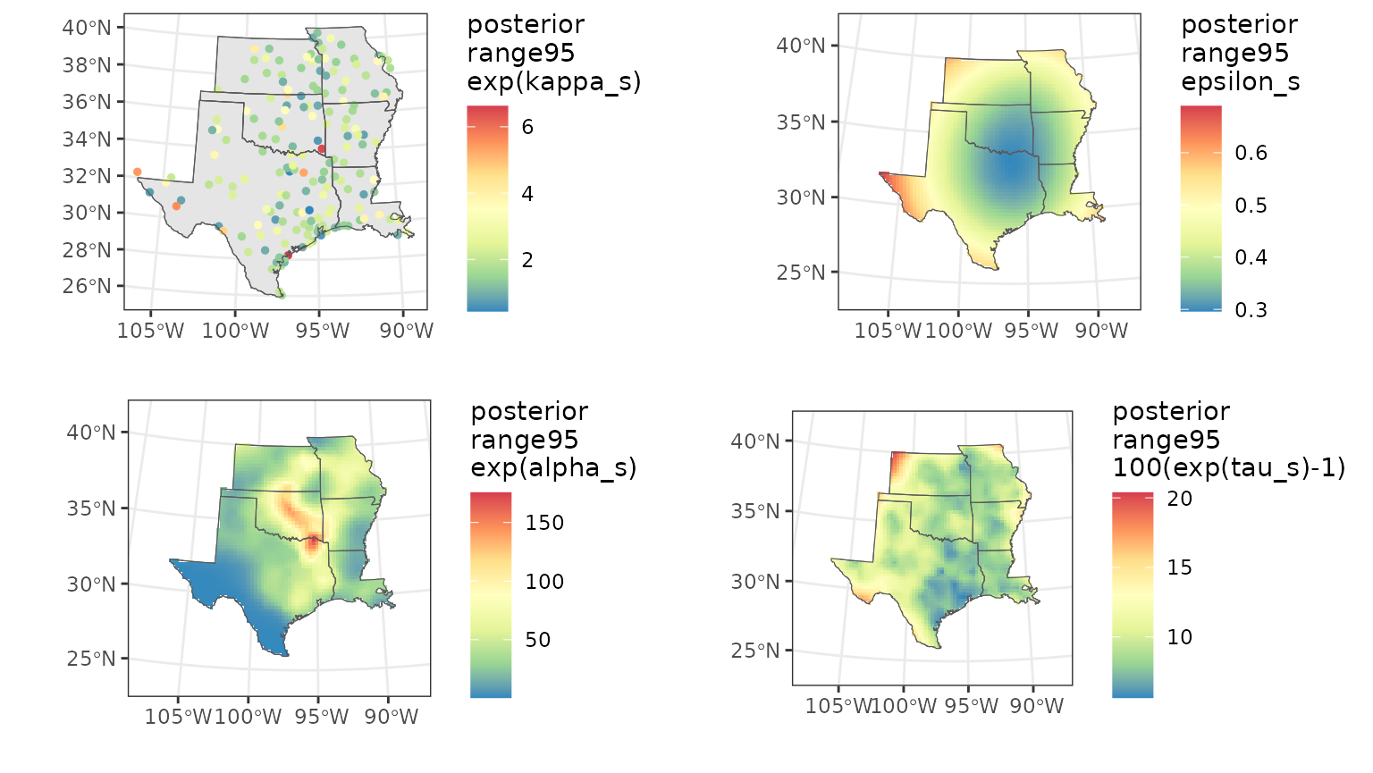
More information
More information on building spatial models using the SPDE approach in R-INLA can be found in Lindgren and Rue (2015), Blangiardo and Camaletti (2015), Bakka et al. (2018), Krainski et al. (2018), and Moraga (2019).
Citations
Bakka, H., Rue, H., Fuglstad, G.A., Riebler, A., Bolin, D., Illian, J., Krainski, E., Simpson, D. and Lindgren, F., 2018. Spatial modeling with R‐INLA: A review. Wiley Interdisciplinary Reviews: Computational Statistics, 10(6), p.e1443.
Besag, J., 1974. Spatial interaction and the statistical analysis of lattice systems. Journal of the Royal Statistical Society: Series B (Methodological), 36(2), pp.192-225.
Blangiardo, M., Cameletti, M., Baio, G. and Rue, H., 2013. Spatial and spatio-temporal models with R-INLA. Spatial and spatio-temporal epidemiology, 4, pp.33-49.
Finley, A.O., 2011. Comparing spatially‐varying coefficients models for analysis of ecological data with non‐stationary and anisotropic residual dependence. Methods in Ecology and Evolution, 2(2), pp.143-154.
Fuglstad, G.A., Simpson, D., Lindgren, F. and Rue, H., 2019. Constructing priors that penalize the complexity of Gaussian random fields. Journal of the American Statistical Association, 114(525), pp.445-452.
Gelfand, A.E., Kim, H.J., Sirmans, C.F. and Banerjee, S., 2003. Spatial modeling with spatially varying coefficient processes. Journal of the American Statistical Association, 98(462), pp.387-396.
Gómez-Rubio, V., 2020. Bayesian inference with INLA. CRC Press.
Krainski, E., Gómez-Rubio, V., Bakka, H., Lenzi, A., Castro-Camilo, D., Simpson, D., Lindgren, F. and Rue, H., 2018. Advanced spatial modeling with stochastic partial differential equations using R and INLA. Chapman and Hall/CRC.
Lindgren, F., Rue, H. and Lindström, J., 2011. An explicit link between Gaussian fields and Gaussian Markov random fields: the stochastic partial differential equation approach. Journal of the Royal Statistical Society: Series B (Statistical Methodology), 73(4), pp.423-498.
Lindgren, F. and Rue, H., 2015. Bayesian spatial modelling with R-INLA. Journal of statistical software, 63, pp.1-25.
Lindgren, F., Bolin, D. and Rue, H., 2022. The SPDE approach for Gaussian and non-Gaussian fields: 10 years and still running. Spatial Statistics, p.100599.
Link, W.A., Sauer, J.R. and Niven, D.K., 2006. A hierarchical model for regional analysis of population change using Christmas Bird Count data, with application to the American Black Duck. The Condor, 108(1), pp.13-24.
Meehan, T.D., Michel, N.L. and Rue, H., 2019. Spatial modeling of Audubon Christmas Bird Counts reveals fine‐scale patterns and drivers of relative abundance trends. Ecosphere, 10(4), p.e02707.
Moraga, P., 2019. Geospatial health data: Modeling and visualization with R-INLA and shiny. CRC Press.
R Core Team (2021). R: A language and environment for statistical computing. R Foundation for Statistical Computing, Vienna, Austria.
Rue, H., Martino, S. and Chopin, N., 2009. Approximate Bayesian inference for latent Gaussian models by using integrated nested Laplace approximations. Journal of the royal statistical society: Series b (statistical methodology), 71(2), pp.319-392.
Simpson, D., Rue, H., Riebler, A., Martins, T.G. and Sørbye, S.H., 2017. Penalising model component complexity: A principled, practical approach to constructing priors. Statistical science, 32(1), pp.1-28.
Soykan, C.U., Sauer, J., Schuetz, J.G., LeBaron, G.S., Dale, K. and Langham, G.M., 2016. Population trends for North American winter birds based on hierarchical models. Ecosphere, 7(5), p.e01351.
Van Niekerk, J. and Rue, H., 2021. Correcting the Laplace Method with Variational Bayes. Journal of Machine Learning Research, Under review.
Van Niekerk, J. and Krainski, E. T. and Rustand, D. and Rue, H., 2022. A new avenue for Bayesian inference with INLA. Submitted.