Blended GEV: a tutorial using R-INLA

Version 1.2

A reparametrisation of the GEV

The blended Generalised extreme value (bGEV) model is an alternative to the usual GEV distribution when the tail parameter $\xi$ is positive, and it is designed to tackle the inherited by the GEV. By artificial boundary restrictions, we mean the following: in practical applications, we assume that the GEV is a reasonable approximation for the distribution of maxima over blocks, and we fit it accordingly. This implies that GEV properties, such as finite lower endpoint in the case $\xi>0$, are inherited by the original maxima distribution, which might not be bounded-supported. This is particularly problematic in the presence of covariates.

Before defining the bGEV distribution, we need to introduce an alternative parametrisation for the GEV. The GEV distribution parametrised in terms of the $q_\alpha\in\mathbb{R}$, the $s_\beta\in(0,\infty)$ and the parameter $\xi\in\mathbb{R}$ has the form

$$F(y\mid q_\alpha,s_\beta,\xi) = \exp\left\{-\left[\left(\frac{y-q_\alpha}{s_\beta(\ell_{1-\beta/2,\xi} - \ell_{\beta/2,\xi})^{-1}} + \ell_{a,\xi}\right)\right]_+^{-1/\xi}\right\},$$ where $a_+=\max(a,0)$ and for any $a>0$, $\ell_{a,\xi} = \{-\log a\}^{-\xi}$. Note that the case $\xi=0$ simplifies to $$F(y\mid q_\alpha,s_\beta) = \exp\left\{-\exp\left[-\left(\frac{y - q_\alpha}{s_\beta(\ell_{1-\beta/2} - \ell_{\beta/2})^{-1}} - \ell_\alpha\right)\right]\right\},$$

with $\ell_a = \log\{-\log a\}.$ There is a one-to-one mapping between $(q_\alpha, s_\beta, \xi)$ and the usual location-scale-shape GEV parameters, $(\mu,\sigma,\xi)$ (see, e.g., Coles, 2001, Chapter 3). For the case $\xi\neq 0$, the mapping is given by

$$\mu=q_\alpha-\frac{s_\beta(\ell_{\alpha,\xi}-1)}{\xi(\ell_{1-\beta/2,\xi} - \ell_{\beta/2,\xi})}, \qquad \sigma = \frac{s_\beta}{(\ell_{1-\beta/2,\xi} - \ell_{\beta/2,\xi})},\qquad\xi = \xi.$$

The case $\xi=0$ is interpreted as the limit when $\xi\to0$, i.e., $$\mu = q_\alpha + \frac{s_\beta\ell_\alpha}{\ell_{\beta/2} - \ell_{1-/\beta/2}},\qquad \sigma = \frac{s_\beta}{\ell_{\beta/2} - \ell_{1-/\beta/2}}.$$

This reparametrisation is proposed to provide a more meaningful interpretation of the parameters. In statistics, the location-scale parametrisation is quite popular as it relates to the mean and the standard deviation of the distribution. In skewed distributions such as the GEV, the mean is no longer a reasonable proxy for the location of the distribution. Moreover, the mean and variance of the GEV are only defined when $\xi<1$ and $\xi<0.5$, respectively. This effect of the tail parameter over the mean and variance does not allow us to interpret the location-scale (and tail) GEV parametrisation as we do in other models. This problem is particularly troublesome for the case where the parameters vary according to a set of covariates. Assigning sensible priors to the GEV distribution with the usual parametrisation is also tricky when the mean and variance are not defined.

The blended GEV model

The bGEV distribution is defined as

$$\begin{equation}\label{eq:bGEV} \text{H}(x \mid \theta) = \text{F}(x \mid q_{\alpha_{\text{F}}}, s_{\beta_{\text{F}}}, \xi)^{p(x \mid s_{p_1}, s_{p_2}, a, b)} \text{G}(x \mid q_{\alpha_{\text{G}}}, s_{\beta_{\text{G}}})^{1-p(x \mid s_{p_1}, s_{p_2}, a, b)}, \end{equation}$$

where $\theta = (q_{\alpha_{\text{F}}}, s_{\beta_{\text{F}}}, \xi, q_{\alpha_{\text{G}}}, s_{\beta_{\text{G}}}, s_{p_1}, s_{p_2}, a, b)$, $\text{F}$ is the Frechét (or type II GEV) distribution with location parameter $q_{\alpha_{\text{F}}}$, spread parameter $s_{\beta_{\text{F}}}$, and parameter $\xi$, and $\text{G}$ is the Gumbel (or type I GEV) distribution with location parameter $q_{\alpha_{\text{G}}}$ and spread parameter $s_{\beta_{\text{G}}}$. The function $p$ is a weight function defined as the cumulative distribution function of a Beta distribution with shape parameters $s_{p_1}>1$ and $s_{p_2}>1$, evaluated in the point $(x - a)/(b - a)$, i.e.,

$$\begin{equation}\label{eq:weightfunction} p(x \mid s_{p_1},s_{p_2}, a, b) = \text{Pr}\left(Y\leq \frac{x-a}{b-a} \mid s_{p_1}, s_{p_2}\right), \end{equation}$$

where $Y$ follows a Beta distribution with shape parameters $s_{p_1}>1$ and $s_{p_2}>1$. The Beta weight controls the way the distributions $\text{F}$ (Frechét) and $\text{G}$ (Gumbel) influence the model $\text{H}$. The lower and upper bounds of the weight function ($a$ and $b$, respectively) define the , i.e., where $F$ and $G$ are merged (see Figure ). Here, we choose them as quantiles of the Frechét distribution, i.e., $a=F^{-1}(p_a)$ and $b=F^{-1}(p_b)$, with $0<p_a,p_b<1$. Below, $p_a$ and $p_b$ will be refered as the . The current INLA implementation assumes that $s_{p_1}=s_{p_2}=5$.

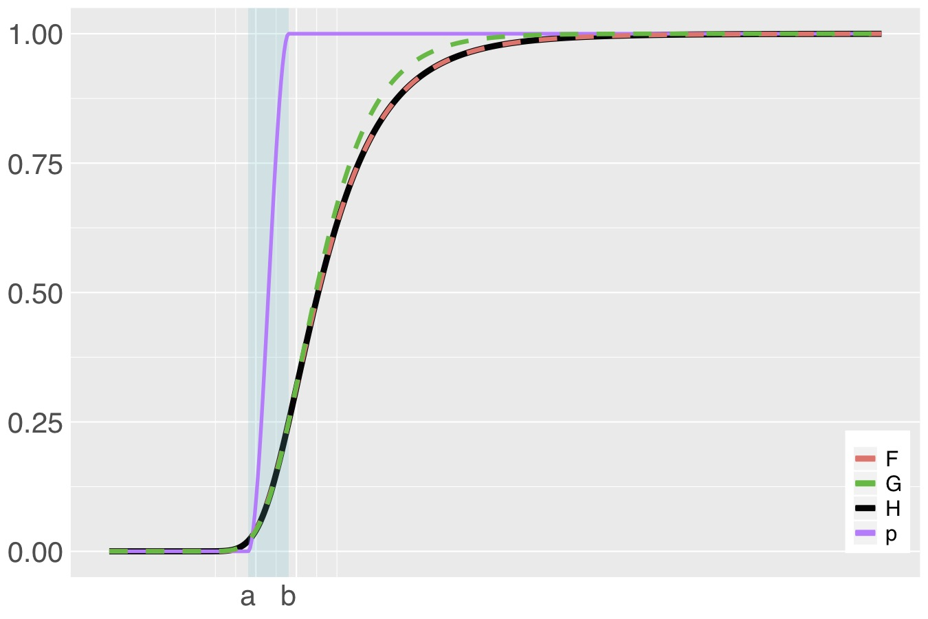
bGEV distribution (H, black) constructed from distributions F (Frechét, red), G (Gumbel, green) and Beta weight function $p$ (purple). The shaded area is the mixing area, where F and G are merged.

In the following sections, we will learn how to fit the bGEV using R-INLA using three simulated examples with increasing level of complexity.

Simulated example 1

To get familiar with the bGEV R-INLA implementation, we consider a simple model where the linear predictor is linked to the $\alpha-$quantile, $q_\alpha$. The model we want to fit is

$$\begin{equation}\label{eq:sim.model1} q_\alpha = \eta(\texttt{x}) = 1 + 0.4\texttt{x} \end{equation}$$

Data simulation

We start by generating $n=1000$ samples from

n = 1000
x = rnorm(n, sd=0.5) # we generate values for x from a N(0,0.5^2) dist.
eta.x = 1 + 0.4*x

The spread and tail parameters are assumed to be covariate-free and unknown and are treated as hyperparameters within the INLA framework. We assume that the true spread and tail parameters are 0.3 and 0.1, respectively.

spread = 0.3
tail = 0.1

To generate the GEV samples, we need to define the probabilities $\alpha$ and $\beta$ that define the location ($q_\alpha$) and spread ($s_\beta$) parameters, respectively. In our case, they will be fixed to $\alpha=0.5$ (the median) and $\beta=0.25$:

p.alpha = 0.5
p.beta = 0.25

Now we are ready to generate the samples. We use the function $\texttt{giveme.gev.par}$ (See Section 5) to obtain the usual GEV parameters ($\mu,\sigma,\xi$) and plug them into the $\texttt{evd::rgev}$ function to generate the samples

par = giveme.gev.par(q = eta.x, sbeta = spread, alpha = p.alpha, beta = p.beta, 
                     xi = tail)
y = numeric(n)
for(i in 1:n) 
  y[i] = rgev(1, loc = par$mu[i], scale = par$sigma, shape = par$xi)

Prior specification

The default prior distribution for the spread $s_\beta$ is a Gamma with shape and rate parameters equal to 3 (note that a log-scale is used below). For the tail parameter we consider a PC prior approach with parameters $\lambda = 7$, $\texttt{low} = 0$ and $\texttt{high}=0.5$. For more details on the PC prior for the tail GEV parameter see Section 4.2.

For the sake of illustration, we here define the priors for all the parameters involved. The priors for the spread is

hyper.spread = list(initial = 1,
                    fixed=FALSE,
                    prior = "loggamma",
                    param = c(3, 3))

The prior for the tail parameter requires a bit more explanation. For computational reasons, R-INLA uses an internal parametrisation of the tail parameter, which is unbounded. The hyperparameter specification is defined for this internal parameter instead of the usual one, so in order to know how to specify a prior for the tail parameter, we need to understand how both parametrisations are connected.

The map $\phi:[0,\infty)\to\mathbb{R}$ specifies the link between the usual and the internal parametrisations and it is defined as $$\phi(\xi_{\text{int}}) = \texttt{low} + (\texttt{high}-\texttt{low})\frac{\exp(\xi_{\text{int}})}{1+\exp(\xi_{\text{int}})}:= \xi,$$ where $\xi\in[0,\infty)$ is the usual tail parameter and $\xi_{\text{int}}$ refers to the unbounded internal tail parameter. The interval $(\texttt{low},\texttt{high})$ constraints the possible values for $\xi$. The map and its inverse are defined in the function $\texttt{map.tail}$ (See Section 5).

In the internal parametrisation, the default initial value is -4 with $(\texttt{low},\texttt{high}) = (0,0.5)$, which correspond to $\xi\approx0.04$. If we want to provide an initial value of $\xi=0.1$, then we can do

tail.interval = c(0, 0.5)
tail.intern = map.tail(tail, tail.interval, inverse=TRUE)

We kept $(\texttt{low},\texttt{high}) = (0,0.5)$ to ensure the existence of second moments.

The prior for the tail parameter is defined as

hyper.tail = list(initial = tail.intern, 
                  prior = "pc.gevtail",
                  param = c(7, tail.interval), 
                  fixed= FALSE)

if we have reasons to believe that $\xi=0$ (Gumbel case), then a good initial value is $-\infty$ (in the internal parametrisation). We can generalise the prior specification for the tail to allow $\xi>0$ or $\xi=0$ as follows

hyper.tail = list(initial = if (tail == 0.0) -Inf else tail.intern, 
                  prior = "pc.gevtail",
                  param = c(7, tail.interval), 
                  fixed= if (tail == 0.0) TRUE else FALSE)

Therefore, the (default) hyperparameter specification for the bGEV model is

hyper.bgev = list(spread = hyper.spread, 
                  tail = hyper.tail)

Control variables

As part of the $\texttt{control.family}$ argument in R-INLA, the argument $\texttt{control.bgev}$ allows us to include additional bGEV parameters. Specifically, the probabilities $\alpha$ and $\beta$, the mixing area quantiles $p_a$ and $p_b$, and the Beta weight function parameters, which we know are equal and fixed to 5 (for now, this cannot be changed).

control.bgev = list(q.location = p.alpha,
                    q.spread = p.beta,
                    # quantile levels for the mixing part
                    q.mix= c(0.05, 0.20), 
                    # the Beta(s1, s2) mixing distribution parameters. 
                    # Hard-coded for the moment: s1=s2=5
                    beta.ab = 5)

INLA fit

The INLA formula for the bGEV model uses the function $\texttt{inla.mdata}$ to allow the inclusion of simple linear models in the spread and the tail parameters (for details on the $\texttt{inla.mdata}$ function see Section 4.3). A null matrix can be used to indicate that these parameters are covariate-free (as it is the case in this example).

null.matrix = matrix(nrow = n, ncol= 0)
spread.x = null.matrix
tail.x = null.matrix

matrices for the spread and tail covariates (here spread.x and tail.x) should always be defined and passed to the R-INLA formula, even if they are empty.

Then, the INLA data and formula can be defined as

data.bgev = data.frame(y = y, intercept = 1, x = x, spread.x = spread.x, tail.x = tail.x)
formula = inla.mdata(y, spread.x, tail.x) ~ -1 + intercept + x

$\texttt{data.bgev}$ only contains three columns, as null matrices cannot be passed to data frames in R. As $\texttt{spread.x}$ and $\texttt{tail.x}$ are not defined in $\texttt{data.bgev}$, INLA will search for these variables in the global R environment. Therefore, $\texttt{spread.x}$ and $\texttt{tail.x}$ should be defined as null matrices in the global environment (as we do here). We write $\texttt{data.bgev}$ this way for consistency with the following examples.

Finally, we fit the model

r1 = inla(formula,
         family = "bgev",
         data = data.bgev,
         control.family = list(hyper = hyper.bgev,
                               control.bgev = control.bgev),
         control.predictor = list(compute = TRUE),
         control.fixed = list(prec=1000),
         control.compute = list(cpo = TRUE),
         control.inla = list(int.strategy = "eb"),
         verbose=FALSE, safe=TRUE)

A summary of the fitted fixed effects and hyperparameters can be obtained as follows

round(r1$summary.fixed,4)

##             mean     sd 0.025quant 0.5quant 0.975quant   mode kld
## intercept 0.9866 0.0031     0.9806   0.9866     0.9926 0.9866   0
## x         0.3798 0.0058     0.3685   0.3798     0.3911 0.3798   0

round(r1$summary.hyperpar,4)

##                                mean     sd 0.025quant 0.5quant 0.975quant
## spread for BGEV observations 0.2838 0.0078     0.2687   0.2837     0.2995
## tail for BGEV observations   0.1085 0.0243     0.0652   0.1070     0.1601
##                                mode
## spread for BGEV observations 0.2836
## tail for BGEV observations   0.1049

Simulated example 2

Although R-INLA does not allow more than one linear predictor, the bGEV implementation does allow for simpler regression models on the spread and tail parameters. We then extend model as follows

$$\begin{align}\label{eq:sim.model2} q_\alpha &= \eta(\texttt{x}_{1}) = 1 + 0.4\texttt{x}_{1}\nonumber\\ s_\beta &= \exp(0.1 + 0.3\texttt{x}_{2})\nonumber\\ \xi &= 0.1 + 0.2\texttt{x}_{3} \end{align}$$

Data simulation

As before, we start by generating $n=1000$ samples from

n = 1000
x1 = rnorm(n)
eta.x = 1 + 0.4*x1

The spread and tail parameter can be simulated as follows

x2 = rnorm(n, sd= 0.2)
s.x = exp(0.1 + 0.3*x2)
x3 = runif(n,-0.25,1)
t.x = 0.1 + 0.2*x3
tail.intern = map.tail(t.x, tail.interval, inverse=TRUE) # internal xi

Note that since $-0.5<\texttt{x}_{3}<2$, we have that $0<\xi<0.5$. As before, we use the function $\texttt{giveme.gev.par}$ to obtain the usual GEV parameters and plug them into the $\texttt{evd::rgev}$ function to generate the samples (note that $\alpha$ and $\beta$ are the same as before)

par = giveme.gev.par(q = eta.x, sbeta = s.x, alpha = p.alpha, beta = p.beta, 
                     xi = t.x)
y = numeric(n)
for(i in 1:n) 
  y[i] = rgev(1, loc = par$mu[i], scale = par$sigma[i], shape = par$xi[i])

Prior specification

Additional to what was discussed in Section 3.2, we can also adjust the priors for the regression coefficient of the covariates for the spread and tail parameters, which we will call $\beta_1$ and $\beta_2$. Within INLA, $\beta_1$ and $\beta_2$ are treated as hyperparameters, with default prior given by a zero-mean Gaussian distribution with precision equal to 300, as specified below.

hyper.beta1 = hyper.beta2 = list(prior = "normal",
                                 param = c(0, 300),
                                 initial = 0)

In this case, the (default) hyperparameter specification for the bGEV model is

hyper.bgev = list(spread = hyper.spread, 
                  tail = hyper.tail,
                  beta1 = hyper.beta1,
                  beta2 = hyper.beta2)

INLA fit

As mentioned in Section 3.4, we can use the $\texttt{inla.mdata}$ function to define linear models for the spread and the tail parameters.

spread.x = x2
tail.x = x3
formula = inla.mdata(y, spread.x, tail.x) ~ -1 + intercept + x

Then, the INLA data can be defined as

data.bgev = data.frame(y = y, intercept = 1, x = x, spread.x = spread.x, tail.x = tail.x)

We fit the model using the same priors and mixing area quantiles ($p_a$, $p_b$) as before.

r2 = inla(formula,
         family = "bgev",
         data = data.bgev,
         control.family = list(hyper = hyper.bgev,
                               control.bgev = control.bgev),
         control.predictor = list(compute = TRUE),
         control.fixed = list(prec=1000),
         control.compute = list(cpo = TRUE),
         control.inla = list(int.strategy = "eb"),
         verbose=FALSE, safe=TRUE)

A summary of the fitted fixed effects and hyperparameters can be obtained as follows

round(r2$summary.fixed,4)

##              mean     sd 0.025quant 0.5quant 0.975quant    mode kld
## intercept  0.7154 0.0178     0.6805   0.7154     0.7504  0.7154   0
## x         -0.0142 0.0257    -0.0646  -0.0142     0.0362 -0.0142   0

round(r2$summary.hyperpar,4)

##                                        mean     sd 0.025quant 0.5quant
## spread for BGEV observations         1.4897 0.0368     1.4188   1.4892
## tail for BGEV observations           0.0364 0.0160     0.0111   0.0344
## beta1 (spread) for BGEV observations 0.0336 0.0526    -0.0700   0.0336
## beta2 (tail) for BGEV observations   0.0008 0.0577    -0.1133   0.0009
##                                      0.975quant   mode
## spread for BGEV observations             1.5637 1.4880
## tail for BGEV observations               0.0716 0.0294
## beta1 (spread) for BGEV observations     0.1370 0.0336
## beta2 (tail) for BGEV observations       0.1138 0.0016

Simulated example 3

The linear predictor can include more complicate structures defined as functions that depend on a set of covariates. By varying the form of these functions, we can accommodate a wide range of models, from standard and hierarchical regression to spatial and spatio-temporal models (Rue et al., 2009). Here we extend the model in by assuming the following structure

$$\begin{align}\label{eq:sim.model3} q_\alpha &= \eta(\texttt{x}_{1},\texttt{z}_{1},\texttt{z}_{2}) = 1 + 0.4\texttt{x}_{1} + f_1(\texttt{z}_{1}) + f_2(\texttt{z}_{2})\nonumber\\ s_\beta &= \exp(0.1 + 0.3\texttt{x}_{2} + \texttt{x}_{4})\nonumber\\ \xi &= 0.1 + 0.2\texttt{x}_{3} \end{align}$$

where $f_1$ is a random walk of order 1 and $f_2$ is an autoregressive process of order 2. Note that we also extended the linear model for the spread parameter.

Data simulation

There are many ways we can simulate dara to fit . One alternative is

n = 1000
x = rnorm(n)
z1 = seq(0, 6, length.out = n)
z2 = 1:n
p = 2 # AR order
pacf = runif(p)
phi = inla.ar.pacf2phi(pacf)
eta.x = 1 + 0.4*x + sin(z1) + c(scale(arima.sim(n, model = list(ar = phi))))

The spread and tail parameter are simulated as before:

x2 = rnorm(n, sd = 0.2)
x4 = rnorm(n, sd = 0.2)
s.x = exp(0.1 + 0.3*x2 + x4)
x3 = runif(n,-0.2, 0.2)
t.x = 0.1 + 0.2*x3
tail.intern = map.tail(t.x, tail.interval, inverse=TRUE) # internal xi

The data are simulated as

par = giveme.gev.par(q = eta.x, sbeta = s.x, alpha = p.alpha, beta = p.beta, 
                     xi = t.x)
y = numeric(n)
for(i in 1:n) 
  y[i] = rgev(1, loc = par$mu[i], scale = par$sigma[i], shape = par$xi[i])

INLA fit

We have two covariates for the spread parameter and one for the tail, and we can have priors for each of their coefficients. Below, $\texttt{hyper.beta1}$ and $\texttt{hyper.beta2}$ are the priors for the coefficients of the covariates in the spread parameters, while $\texttt{hyper.beta3}$ is the prior for the coefficient of the covariate in the tail parameter.

hyper.beta1 = hyper.beta2 = hyper.beta3 = list(prior = "normal",
                                               param = c(0, 300),
                                               initial = 0)
hyper.bgev = list(spread = hyper.spread, 
                  tail = hyper.tail,
                  beta1 = hyper.beta1,
                  beta2 = hyper.beta2,
                  beta3 = hyper.beta3)

Using the same mixing area quantiles ($q_a$, $q_b$) as before, we only need to specify the INLA formula, the new data, and run the model.

spread.x = x2
spread.xx = x4
tail.x = x3
# With this change of variable it is easier to keep track of the effect 
# of the covariates in each parameter, but it is not needed.
formula = inla.mdata(y, cbind(spread.x, spread.xx), tail.x) ~ -1 + intercept + x + 
    f(z1, model = "rw1", scale.model=TRUE, constr=TRUE,
        hyper = list(prec = list(prior = "pc.prec", 
        param = c(0.1, 0.01)))) +
    f(z2, model = 'ar', order = 1, 
           hyper=list(prec=list(prior="pc.prec", constr=TRUE,
                                param=c(0.1,0.01)),
                      pacf1=list(param=c(0.5,0.8),
                      pacf2=list(param=c(0.5,0.8)))))
data.bgev = data.frame(y = y, intercept = 1, x = x, z1 = z1, z2 = z2,
                       spread.x = spread.x, spread.xx = spread.xx, tail.x = tail.x)
r3 = inla(formula,
         family = "bgev",
         data = data.bgev,
         control.family = list(hyper = hyper.bgev,
                               control.bgev = control.bgev),
         control.predictor = list(compute = TRUE),
         control.fixed = list(prec=1000,prec.intercept=1000),
         control.compute = list(cpo = TRUE),
         control.inla = list(int.strategy = "eb",
                             cmin=0,
                             b.strategy="keep"),
         verbose=FALSE, safe=TRUE)

A summary of the fitted effects and hyperparameters can be obtained as follows

round(r3$summary.fixed,4)

##             mean     sd 0.025quant 0.5quant 0.975quant   mode kld
## intercept 0.0220 0.0313    -0.0392   0.0220     0.0833 0.0220   0
## x         0.2188 0.0212     0.1772   0.2188     0.2604 0.2188   0

round(r3$summary.hyperpar,4)

##                                            mean         sd 0.025quant  0.5quant
## spread for BGEV observations             2.1125     0.0665     1.9858    2.1110
## tail for BGEV observations               0.0065     0.0077     0.0004    0.0041
## beta1 (spread) for BGEV observations     0.0379     0.0535    -0.0681    0.0381
## beta2 (spread) for BGEV observations     0.0397     0.0536    -0.0650    0.0394
## beta3 (tail) for BGEV observations      -0.0001     0.0577    -0.1139    0.0000
## Precision for z1                     18295.3465 77385.5575    12.2080 2712.4478
## Precision for z2                         1.1787     0.1588     0.8971    1.1681
## PACF1 for z2                             0.9621     0.0064     0.9484    0.9625
##                                       0.975quant   mode
## spread for BGEV observations              2.2477 2.1072
## tail for BGEV observations                0.0273 0.0011
## beta1 (spread) for BGEV observations      0.1427 0.0390
## beta2 (spread) for BGEV observations      0.1459 0.0384
## beta3 (tail) for BGEV observations        0.1135 0.0002
## Precision for z1                     130615.0703 0.6250
## Precision for z2                          1.5213 1.1472
## PACF1 for z2                              0.9735 0.9631

Notes

Linear predictor for the bGEV model

The linear predictor can take any combinations of the latent structures currently implemented. To see a list of the available latent models, we can do

library(INLA)
inla.list.models('latent')

PC prior for the tail parameter

Although non-informative priors are a common choice when little expert knowledge is available, the PC prior approach allows us to select moderately informative prior distributions in a $\textit{reasonable}$ way. This procedure penalises excessively complex models at a constant rate by putting an exponential prior on a distance (specifically, the Kullback-Leibler distance, or KLD) to a simpler baseline model.

The PC prior for the tail GEV parameter is defined in terms of the KLD $\xi^2/(1-\xi)$ for $0\leq \xi<1$. In R-INLA, the prior is specified as $$\texttt{hyper = list(<theta> = list(prior="pc.gevtail", param=c(<lambda>, <low>, <high>)))}$$ where

• $\texttt{<lambda>}$: the constant penalisation rate
• $\texttt{<low>,<high>}$: interval to restrict possible values for the tail parameter. The default is [0,0.5].

For more details on the PC prior for the tail GEV parameter see $\texttt{inla.doc("pc.gevtail")}$.

About $\texttt{inla.mdata}$

$\texttt{inla.mdata(y, x1, x2,...)}$ is a matrix where each row are replicates, and responses that are $\texttt{NA}$s are ignored. The function $\texttt{inla.mdata}$ accept covariates that are one or many vectors, matrices or data frames. If we pass $m$ covariates $\texttt{x}_1,\ldots\texttt{x}_m$, then each row $(\texttt{x}_{i1}, \texttt{x}_{i2}, \ldots, \texttt{x}_{im})$ defines the covariates used for the $i$-th row of $\texttt{y}$.

Tools

The function $\texttt{giveme.gev.par}$ computes the usual GEV parameters $(\mu,\sigma,\xi)$ given the bGEV parameters $(q,s_\beta,\xi)$. Note that in both parametrisations, the tail parameter is the same.

library(evd)
giveme.gev.par = function(q, sbeta, alpha, beta, xi) 
{
  .mu = function(q, sbeta, alpha, beta, xi) {
    a = -log(1-beta/2)
    b = -log(beta/2)
    c = -log(alpha)
    if (all(xi > 0.0)) {
      tmp0 = (c^(-xi) - 1)/xi
      tmp1 = a^(-xi)
      tmp2 = b^(-xi)
      dbeta = (tmp1 - tmp2)/xi
      return(q - (sbeta/dbeta) * tmp0)
    } else if (all(xi == 0.0)) {
      dbeta = log(b) - log(a)
      tmp0 = log(c)
      return(q + (sbeta/dbeta) * tmp0)
    } else {
      stop("mixed case not implemented")
    }
  }
  
  .sigma = function(q, sbeta, alpha, beta, xi) {
    a = -log(1-beta/2)
    b = -log(beta/2)
    if (all(xi > 0.0)) {
      tmp1 = a^(-xi)
      tmp2 = b^(-xi)
      dbeta = (tmp1 - tmp2)/xi
      return(sbeta/dbeta)
    } else if (all(xi == 0.0)) {
      dbeta = log(b) - log(a)
      return(sbeta/dbeta)
    } else {
      stop("mixed case not implemented")
    }
  }
  
  return(list(mu = .mu(q, sbeta, alpha, beta, xi),
              sigma = .sigma(q, sbeta, alpha, beta, xi),
              xi = xi))
}

The function $\texttt{map.tail}$ specifies the link between the internal and usual parametrisations. In the code below, $\texttt{interval}$ constraints the possible values for the tail parameter, while $\texttt{inverse}$ is a boolean variable indicating whether $\phi$ or $\phi^{-1}$ should be computed.

map.tail = function(x, interval, inverse = FALSE) {
  if (!inverse) {
    return (interval[1] + (interval[2] - interval[1]) * exp(x)/(1.0 + exp(x)))
  } else {
    return (log((x-interval[1])/(interval[2]-x)))
  }
}

1. Coles, S. (2001). (Vol. 208, p. 208). London: Springer.

2. Rue, H., Martino, S., & Chopin, N. (2009). Approximate Bayesian inference for latent Gaussian models by using integrated nested Laplace approximations. , 71(2), 319-392.