Fitting CoDa using the Logistic Gaussian distribution with Dirichlet covariance structure
Version 1.0.0
2026-04-04 16:35:39.436903
Dirichlet-CoDa.RmdAn introduction to the Logistic Normal Dirichlet Regression
As defined in Martínez-Minaya and Rue (2023), follows a logistic-normal distribution with Dirichlet covariance if and only if , and: where represents the variance of each log-ratio and is the covariance between log-ratios. From now on we will refer to as the multivariate normal with Dirichlet covariance structure.
Let be a multivariate random variable such as , which by definition is equivalent to . Because of its easy interpretability in terms of log-ratios with the reference category, we focus on modelling as a .
Simulated example I (Type II)
The model with which we are going to operate in this example presents the following structure:
Note that this is the second structure presented in Martínez-Minaya and Rue (2023), where we are working under the assumption that covariates have different effect in each linear predictor. In particular, we consider , and the reference category is the third one. So, we are dealing with two -coordinates. Also, we just generate a covariate scaled to have mean 0 and standard deviation 1.
Data simulation
set.seed(201803)
inla.seed = sample.int(n=1E6, size=1)
options(width=70, digits=3)
Defining hyperparameters and dimensionality of the response
We start defining the hyperparameters of the likelihood: , and , and computing the correlation matrix of the -coordinates.
### --- 1. Simulation --- ####
# Parameters for the simulation
D <- 3
N <- 1000
sigma2 <- c(0.5, 0.4)
cov_param <- 0.1
sigma_diag <- sqrt(sigma2 + cov_param)
hypers_lik <- data.frame(hypers = c(sigma2, cov_param),
                         name1 = c("sigma2.1", "sigma2.2", "gamma"))
# We create the correlation parameters based on the previous idea
# We are going to have ((D-1)^2 - (D-1))/2 rhos
rho <- diag(1/sigma_diag) %*% matrix(cov_param, D-1, D-1) %*% diag(1/sigma_diag)
diag(rho) <- 1
rho
## [,1] [,2]
## [1,] 1.000 0.183
## [2,] 0.183 1.000Simulating a covariate
We define the covariate and also, the corresponding betas, constructing the corresponding linear predictor.
Data in the simplex
We move back to the Simplex using the
-inverse,
in particular, we use the function alrInv form the
R-package compositions.
  y.simplex <- compositions::alrInv(alry)
  y.simplex <- as.numeric(t(y.simplex)) %>% matrix(., ncol = D, byrow = TRUE)
  colnames(y.simplex) <- paste0("y", 1:D)
  data <- data.frame(alry, y.simplex, x)
colnames(data)[1:(D-1)] <- c(paste0("alry.", 1:(D-1)))
data %>% head(.)
## alry.1 alry.2 y1 y2 y3 x
## 1 -1.580 -1.46 0.143 0.1620 0.695 0.0265
## 2 -1.345 -3.18 0.200 0.0318 0.768 -0.3708
## 3 -1.735 -1.52 0.126 0.1567 0.717 0.0819
## 4 -1.012 -2.01 0.243 0.0898 0.667 -0.0377
## 5 -0.584 -1.53 0.314 0.1224 0.563 0.0775
## 6 -0.041 2.10 0.095 0.8060 0.099 0.3962Plotting the simulated data
### Alr coordinates
data %>%
  tidyr::pivot_longer(., cols = ,starts_with("alr"),
                      names_to = "y.names", values_to = "y.resp") %>%
  ggplot(data = .) +
  geom_point(aes(x = x, y = y.resp, fill = x), shape = 21, size = 2) +
  ylab("alr") +
  facet_wrap(~y.names) +
  theme_bw() +
  theme(legend.position = "bottom") -> p_alr

#pdf("simulated_data.pdf", width = 8, height = 6)
p_alr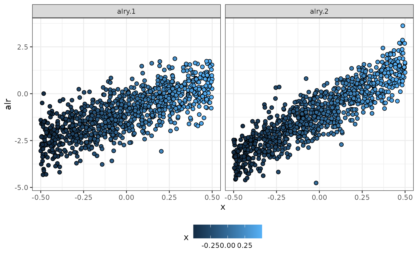
Simulated data using alr-coordinates in terms of x
#dev.off()Data preparation for fitting
Index for individual
data$id.z <- 1:dim(data)[1]Extending the dataset
We extent the data with
-coordinates
for introducing in inla.stack
data_ext <- data %>%
  tidyr::pivot_longer(., cols = all_of(paste0("alry.", 1:(D-1))),
                      names_to  = "y.names",
                      values_to = "y.resp") %>%
  .[order(ordered(.$y.names)),]
data_ext$y.names <- ordered(data_ext$y.names)
head(data_ext)
## # A tibble: 6 × 7
## y1 y2 y3 x id.z y.names y.resp
## <dbl> <dbl> <dbl> <dbl> <int> <ord> <dbl>
## 1 0.143 0.162 0.695 0.0265 1 alry.1 -1.58
## 2 0.200 0.0318 0.768 -0.371 2 alry.1 -1.35
## 3 0.126 0.157 0.717 0.0819 3 alry.1 -1.74
## 4 0.243 0.0898 0.667 -0.0377 4 alry.1 -1.01
## 5 0.314 0.122 0.563 0.0775 5 alry.1 -0.584
## 6 0.0950 0.806 0.0990 0.396 6 alry.1 -0.0410Response in R-INLA
We create a matrix with dimension
for including the multivariate response in R-INLA
names_y <- paste0("alry.", 1:(D-1))
1:length(names_y) %>%
  lapply(., function(i){
    data_ext %>%
      dplyr::filter(y.names == names_y[i]) -> data_comp_i
    #Response
    y_alr <- matrix(ncol = names_y %>% length(.), nrow = dim(data_comp_i)[1])
    y_alr[, i] <- data_comp_i$y.resp
  }) -> y.resp

1:length(names_y) %>%
  lapply(., function(i){
    y_aux <- data_ext %>%
      dplyr::select(y.resp, y.names) %>%
      dplyr::filter(y.names == names_y[i]) %>%
      dplyr::select(y.resp) %>%
      as.matrix(.)
    aux_vec <- rep(NA, (D-1))
    aux_vec[i] <- 1
    kronecker(aux_vec, y_aux)
  }) -> y_list

y_tot <- do.call(cbind, y_list)
y_tot %>% head(.)
## [,1] [,2]
## [1,] -1.580 NA
## [2,] -1.345 NA
## [3,] -1.735 NA
## [4,] -1.012 NA
## [5,] -0.584 NA
## [6,] -0.041 NACovariates in R-INLA
Covariates are going to be included in the model as random effects with big variance. So, we need the values of the covariates, and also, an index indicating to which alr-coordinate it belongs.
variables <- c("intercept", data %>%
                 dplyr::select(starts_with("x")) %>%
                 colnames(.))
id.names <- paste0("id.", variables)
id.variables <- rep(data_ext$y.names %>% as.factor(.) %>% as.numeric(.),
                    length(variables)) %>%
  matrix(., ncol = length(variables), byrow = FALSE)
colnames(id.variables) <- id.names

variables
## [1] "intercept" "x"## id.intercept id.x
## [1,] 1 1
## [2,] 1 1
## [3,] 1 1
## [4,] 1 1
## [5,] 1 1
## [6,] 1 1
inla.stack
We create an inla.stack for estimation
stk.est <- inla.stack(data    = list(resp = y_tot),
                      A       = list(1),
                      effects = list(cbind(data_ext %>%
                                             dplyr::select(starts_with("x")),
                                           data_ext %>%
                                             dplyr::select(starts_with("id.z")),
                                           id.variables,
                                           intercept = 1)),
                      tag     = 'est')
Fitting the model
In this section, we fit a model (Type II in the manuscript), and we obtain the marginal posterior distribution of the parameters and hyperparameters
Fit in R-INLA
  # Have different parameters for fixed effects, and do not include spatial random effects.
list_prior <- rep(list(list(prior = "pc.prec", param = c(1, 0.01))), D-1)

### Fitting the model
formula.typeII <- resp ~ -1 +
  f(id.intercept, intercept,
    model   = "iid",
    initial = log(1/1000),
    fixed   = TRUE) +
  f(id.x, x,
    model   = "iid",
    initial = log(1/1000),
    fixed   = TRUE) +
  f(id.z,
    model = "iid",
    hyper = list(prec = list(prior = "pc.prec",
                             param = c(1, 0.01))), constr = TRUE)
model.typeII <- inla(formula.typeII,
                     family         = rep("gaussian", D-1),
                     data           = inla.stack.data(stk.est),
                     control.compute = list(config = TRUE),
                     control.predictor = list(A = inla.stack.A(stk.est),
                                              compute = TRUE),
                     control.family = list_prior,
                     inla.mode = "experimental" ,
                     verbose = FALSE)
Marginal posterior distribution of the fixed effects
### Posterior distribution of the fixed effects
data_fixed <- rbind(data.frame(inla.smarginal(model.typeII$marginals.random$id.x$index.1),
                               alr = "alr(y1/y3)",
                               var = "x",
                               param = "beta1",
                               real  = betas[1,2]),
                    data.frame(inla.smarginal(model.typeII$marginals.random$id.x$index.2),
                               alr = "alr(y2/y3)",
                               var = "x",
                               param = "beta1",
                               real  = betas[2,2]),
                    data.frame(inla.smarginal(model.typeII$marginals.random$id.intercept$index.1),
                               alr = "alr(y1/y3)",
                               var = "intercept",
                               param = "beta0",
                               real = betas[1,1]),
                    data.frame(inla.smarginal(model.typeII$marginals.random$id.intercept$index.2),
                               alr = "alr(y2/y3)",
                               var = "intercept",
                               param = "beta0",
                               real = betas[2,1]))

p_fixed <- ggplot() +
  geom_line(data = data_fixed, aes(x = x, y = y), size = 0.9) +
  #ggtitle("Effect of the covariate bio12") +
  theme_bw() +
  geom_vline(data = data_fixed, aes(xintercept = real), col = "red4") +
 # scale_color_manual(values=c("#E75F00", "#56B4E9"))+
  theme(legend.position = "bottom") +
  facet_wrap(~param + alr, ncol = D-1, scales = "free") +
  xlab(expression(beta^(d))) +
  ylab(expression(p(beta^(d) *'|'* theta))) +
  theme(legend.title = element_blank())

#pdf("posterior_fixed.pdf", width = 6, height = 5)
p_fixed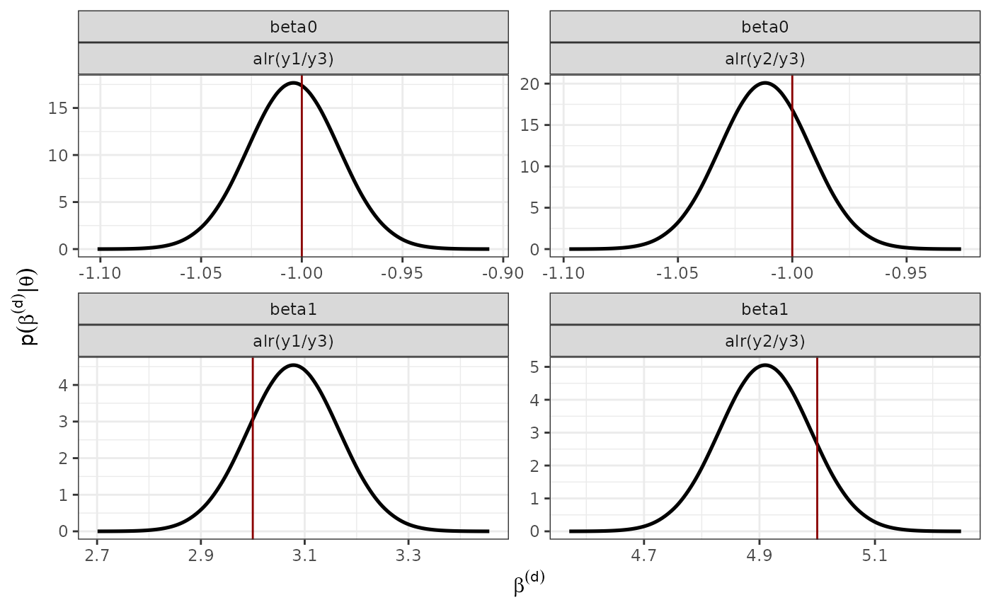
#dev.off()Marginal Posterior distribution of the hyperparameters
### Posterior distribution of the hyperparameters
prec <- list(sigma2.1 = model.typeII$marginals.hyperpar$`Precision for the Gaussian observations`,
             sigma2.2 = model.typeII$marginals.hyperpar$`Precision for the Gaussian observations[2]`,
             gamma = model.typeII$marginals.hyper$`Precision for id.z`)

hyper <- lapply(1:length(prec),
                function(x){
                  inla.smarginal(inla.tmarginal(prec[[x]], fun = function(y)(1/y))) %>%
                    data.frame(.)
                })
names(hyper) <- names(prec)

hyper.df <- lapply(1:length(hyper),
                   function(x){
                     cbind(data.frame(hyper[[x]]), name1 = names(hyper)[x])
                   })  %>%
  do.call(rbind.data.frame, .)

hyper.df$name1 <- ordered(hyper.df$name1,
                          levels = c("sigma2.1", "sigma2.2",
                                     "gamma"))
p.hyper <- ggplot(hyper.df) +
  geom_line(aes(x = x, y = y)) +
  geom_vline(data = hypers_lik, aes(xintercept = hypers), col = "red4") +
  facet_wrap(~ name1, scales = "free") +
  theme_bw() +
  xlab(expression(theta)) +
  ylab(expression(p(theta*'|'*y)))

#pdf("marginals_hyperpar.pdf", width = 6, height = 3)
print(p.hyper)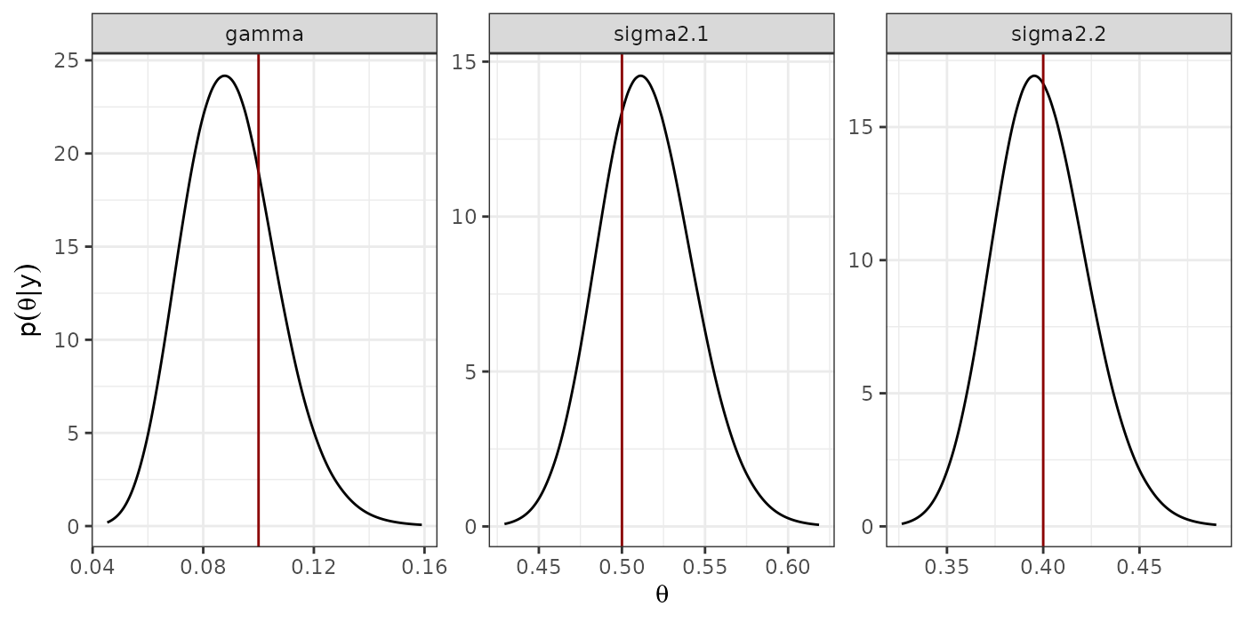
#dev.off()Predicting for a new observation
This section, is devoted to explain how to make predictions. We want to predict, for the values of the covariate . In particular, we show how to compute the posterior preditive distribution for the mean of the -coordinates. Posteriorly, we move back to the Simplex.
Preparing dataset for predictions
sim <- 1000
x.pred <- seq(-0.5, 0.5, 0.3)
n.pred <- length(x.pred)
cat("\n ----------------------------------------------- \n")
##
## -----------------------------------------------
cat("Creating the data.frame for predictions \n")## Creating the data.frame for predictions
data_pred <- data.frame(intercept = 1,
                        x = rep(x.pred, D-1))
id.z.pred  <- rep((N + 1):(N + n.pred), D - 1) #random effect z to model the correlation

# Category
id.cat_pred <- rep(1:(D - 1), rep(n.pred, D - 1))
#Index for covariates
variables_pred <- c("intercept", data_pred %>%
                      dplyr::select(starts_with("x")) %>%
                      colnames(.))
id.names_pred <- paste0("id.", variables_pred)
id.variables_pred <- rep(id.cat_pred, length(variables_pred)) %>%
  matrix(., ncol = length(variables_pred), byrow = FALSE)
colnames(id.variables_pred) <- id.names_pred
Preparing inla.stack for predictions
stk.pred <- inla.stack(data    = list(resp = matrix(NA, ncol = D - 1,
                                                    nrow = n.pred*(D - 1))),
                       A       = list(1),
                       effects = list(cbind(data_pred,
                                            id.z = id.z.pred,
                                            id.variables_pred)),
                       tag     = 'pred')
### --- Total stack
stk <- inla.stack(stk.est, stk.pred)
Prediction
mod.pred <- inla(formula.typeII,
                 family         = rep("gaussian", D - 1),
                 data              = inla.stack.data(stk),
                 control.compute   = list(config = TRUE),
                 control.predictor = list(A = inla.stack.A(stk), compute = TRUE, link = 1),
                 control.mode      = list(theta = model.typeII$mode$theta, restart = TRUE),
                 control.family = list_prior,
                 num.threads       = 2,
                 inla.mode = "experimental" ,
                 verbose           = FALSE)
Extracting predictions using inla.posterior.sample
pred.values.mean <- mod.pred$summary.fitted.values$mean[inla.stack.index(stk, 'pred')$data] %>%
  matrix(., ncol = D - 1, byrow = FALSE)

post_sim_pred <- inla.posterior.sample(n = sim, result = mod.pred)
post_sim_predictor <- inla.posterior.sample.eval(fun = function(...){
  APredictor}, post_sim_pred, return.matrix = TRUE)
post_sim_idz <- inla.posterior.sample.eval(fun = function(...){
  id.z}, post_sim_pred, return.matrix = TRUE)

ind.pred <- inla.stack.index(stk, 'pred')$data
ind.idz <- inla.stack.index(stk, 'est')$data #This is the shared random effect
ind.idz <- ind.idz[1:(length(ind.idz)/(D - 1))]

post_sim_predictor[ind.pred, ] <- post_sim_predictor[ind.pred, ]-
  kronecker(rep(1, D-1), post_sim_idz[-ind.idz,])

post_sim_pred_alr <- post_sim_predictor[ind.pred,]

#Computing mean and sd
pred_alr_summary <- t(apply(post_sim_pred_alr, 1, function(x){c(mean(x), sd(x))}))
pred_alr_summary <- data.frame(pred_alr_summary,
                               y.names = rep(names_y, rep(n.pred, D-1)),
                               x.pred = rep(x.pred, D-1))
colnames(pred_alr_summary)[1:2] <- c("mean", "sd")

pred_alr_summary
## mean sd y.names x.pred
## fun[2001] -2.546 0.0483 alry.1 -0.5
## fun[2002] -1.622 0.0280 alry.1 -0.2
## fun[2003] -0.697 0.0250 alry.1 0.1
## fun[2004] 0.227 0.0429 alry.1 0.4
## fun[2005] -3.467 0.0445 alry.2 -0.5
## fun[2006] -1.994 0.0257 alry.2 -0.2
## fun[2007] -0.520 0.0218 alry.2 0.1
## fun[2008] 0.953 0.0376 alry.2 0.4Predictions in the simplex
###  Prediction in the simplex --- #####
apply(post_sim_predictor[ind.pred,], 2, function(x){
  alr_pred <- matrix(x, ncol = D - 1)
  pred_simplex <- compositions::alrInv(alr_pred)
  as.numeric(t(pred_simplex)) #Byrows
}) -> post_sim_pred_simplex

#Computing credible intervals
pred_simplex_summary <- t(apply(post_sim_pred_simplex, 1, function(x){c(mean(x), sd(x))}))
pred_simplex_summary <- data.frame(pred_simplex_summary,
                                   y.names = rep(c("y1", "y2", "y3"), n.pred),
                                   x.pred  = rep(x.pred, rep(D, n.pred)))
colnames(pred_simplex_summary)[1:2] <- c("mean", "sd")

pred_simplex_summary
## mean sd y.names x.pred
## 1 0.0707 0.00316 y1 -0.5
## 2 0.0282 0.00121 y2 -0.5
## 3 0.9011 0.00340 y3 -0.5
## 4 0.1482 0.00354 y1 -0.2
## 5 0.1021 0.00238 y2 -0.2
## 6 0.7497 0.00376 y3 -0.2
## 7 0.2381 0.00473 y1 0.1
## 8 0.2840 0.00470 y2 0.1
## 9 0.4779 0.00414 y3 0.1
## 10 0.2590 0.00921 y1 0.4
## 11 0.5347 0.01047 y2 0.4
## 12 0.2063 0.00498 y3 0.4