Functions which operates on marginals
marginal.RdDensity, distribution function, quantile function, random generation,
hpd-interval, interpolation, expectations, mode and transformations of
marginals obtained by inla or inla.hyperpar(). These
functions computes the density (inla.dmarginal), the distribution function
(inla.pmarginal), the quantile function (inla.qmarginal), random generation
(inla.rmarginal), spline smoothing (inla.smarginal), computes expected
values (inla.emarginal), computes the mode (inla.mmarginal), transforms the
marginal (inla.tmarginal), and provide summary statistics (inla.zmarginal).
inla.smarginal(
  marginal,
  log = FALSE,
  extrapolate = 0,
  keep.type = FALSE,
  factor = 15L
)

inla.emarginal(fun, marginal, ...)

inla.dmarginal(x, marginal, log = FALSE)

inla.pmarginal(q, marginal, normalize = TRUE, len = 2048L)

inla.qmarginal(p, marginal, len = 2048L)

inla.hpdmarginal(p, marginal, len = 2048L)

inla.rmarginal(n, marginal)

inla.tmarginal(
  fun,
  marginal,
  n = 2048L,
  h.diff = .Machine[["double.eps"]]^(1/3),
  method = c("quantile", "linear")
)

inla.mmarginal(marginal)

inla.zmarginal(marginal, silent = FALSE)

inla.is.marginal(marginal)
Arguments
- marginal
A marginal object from either
inlaorinla.hyperpar(), which is eitherlist(x=c(), y=c())with density valuesyat locationsx, or amatrix(,n,2)for which the density values are the second column and the locations in the first column. Theinla.hpdmarginal()-function assumes a unimodal density.- log
Return density or interpolated density in log-scale?
- extrapolate
How much to extrapolate on each side when computing the interpolation. In fraction of the range.
- keep.type
If
FALSEthen return alist(x=, y=), otherwise ifTRUE, then return a matrix if the input is a matrix- factor
The number of points after interpolation is
factortimes the original number of points; which is argumentninspline- fun
A (vectorised) function like
function(x) exp(x)to compute the expectation against, or which define the transformation new = fun(old)- ...
Further arguments to be passed to function which expectation is to be computed.
- x
Evaluation points
- q
Quantiles
- normalize
Renormalise the density after interpolation?
- len
Number of locations used to interpolate the distribution function.
- p
Probabilities
- n
The number of observations. If
length(n) > 1, the length is taken to be the number required.- h.diff
The step-length for the numerical differeniation inside
inla.tmarginal- method
Which method should be used to layout points for where the transformation is computed.
- silent
Output the result visually (TRUE) or just through the call.
Value
inla.smarginal returns list=c(x=c(), y=c()) of
interpolated values do extrapolation using the factor given, and the
remaining function returns what they say they should do.
See also
Examples
## a simple linear regression example
n = 10
x = rnorm(n)
sd = 0.1
y = 1+x + rnorm(n,sd=sd)
res = inla(y ~ 1 + x, data = data.frame(x,y),
control.family=list(initial = log(1/sd^2L),fixed=TRUE))
## chose a marginal and compare the with the results computed by the
## inla-program
r = res$summary.fixed["x",]
m = res$marginals.fixed$x
## compute the 95% HPD interval
inla.hpdmarginal(0.95, m)
#> low high
#> level:0.95 0.9518712 1.074671
x = seq(-6, 6, length.out = 1000)
y = dnorm(x)
inla.hpdmarginal(0.95, list(x=x, y=y))
#> low high
#> level:0.95 -1.962892 1.95703
## compute the the density for exp(r), version 1
r.exp = inla.tmarginal(exp, m)
## or version 2
r.exp = inla.tmarginal(function(x) exp(x), m)
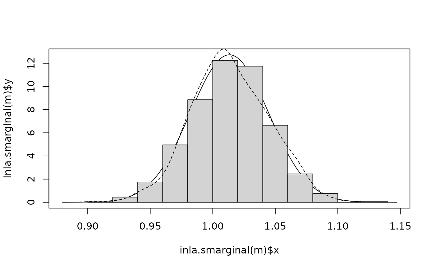
## to plot the marginal, we use the inla.smarginal, which interpolates (in
## log-scale). Compare with some samples.
plot(inla.smarginal(m), type="l")
s = inla.rmarginal(1000, m)
hist(inla.rmarginal(1000, m), add=TRUE, prob=TRUE)
lines(density(s), lty=2)
 m1 = inla.emarginal(function(x) x, m)
m2 = inla.emarginal(function(x) x^2L, m)
stdev = sqrt(m2 - m1^2L)
q = inla.qmarginal(c(0.025,0.975), m)
## inla-program results
print(r)
#> mean sd 0.025quant 0.5quant 0.975quant mode kld
#> x 1.013337 0.03133688 0.9519175 1.013337 1.074756 1.013337 0
## inla.marginal-results (they shouldn't be perfect!)
print(c(mean=m1, sd=stdev, "0.025quant" = q[1], "0.975quant" = q[2L]))
#> mean sd 0.025quant 0.975quant
#> 1.01333663 0.03132028 0.95187122 1.07467146
## using the buildt-in function
inla.zmarginal(m)
#> Mean 1.01334
#> Stdev 0.0313203
#> Quantile 0.025 0.951871
#> Quantile 0.25 0.992139
#> Quantile 0.5 1.01327
#> Quantile 0.75 1.0344
#> Quantile 0.975 1.07467
m1 = inla.emarginal(function(x) x, m)
m2 = inla.emarginal(function(x) x^2L, m)
stdev = sqrt(m2 - m1^2L)
q = inla.qmarginal(c(0.025,0.975), m)
## inla-program results
print(r)
#> mean sd 0.025quant 0.5quant 0.975quant mode kld
#> x 1.013337 0.03133688 0.9519175 1.013337 1.074756 1.013337 0
## inla.marginal-results (they shouldn't be perfect!)
print(c(mean=m1, sd=stdev, "0.025quant" = q[1], "0.975quant" = q[2L]))
#> mean sd 0.025quant 0.975quant
#> 1.01333663 0.03132028 0.95187122 1.07467146
## using the buildt-in function
inla.zmarginal(m)
#> Mean 1.01334
#> Stdev 0.0313203
#> Quantile 0.025 0.951871
#> Quantile 0.25 0.992139
#> Quantile 0.5 1.01327
#> Quantile 0.75 1.0344
#> Quantile 0.975 1.07467