User defined integration points

Introduction

This short note describe a new option that allow the user to use user-defined integration points (or “design” points), instead of the default ones. The relevant integration in INLA does $\int f(x | \theta, y) \; \pi(\theta | y) \; d\theta = f(x | y)$ where $\pi(\theta | y)$ is the approximated posterior marginal for the hyperparameters, and where $f(x | \theta, y)$ is the approximated marginal for $x$ for that configuration. The output of this integral is the posterior marginal $f(x|y)$ . In practice, we use a discrete set of integration points for $\theta$ , and corresponding weights $w$ , to get $f(x|y) \approx \sum_i f(x|\theta_i, y) w_i \pi(\theta_i | y)$ for which we require $w_i \ge 0$ and $\sum_i w_i = 1$ . Usually, the integration is done in a standardised scale, $z = A(\theta - \gamma)$ i.e. with respect to $\pi(z|y)$ . Here, $\gamma$ is the mode of $\pi(\theta|y)$ and the matrix $A$ is the negative square root of the approximated covariance matrix for $\theta|y$ at the mode.

The relevant options are

    opts = control.inla(int.strategy = "user", int.design = Design)

where Design is a matrix with the integration points and the integration weights. The $j$ th row of Design consists of the values $\theta_j = (\theta_{1j}, \ldots, \theta_{mj})$ , and the integration weight for this configuration, $w_j$ . The values are in the $\theta$ -scale, meaning that you have to know exactly what you are doing, including knowing the ordering of the hyperparameters.

Another version, is to define the points in the standardised scale $z$ . To do this, use

    opts = control.inla(int.strategy = "user.std", int.design = Design)

instead. The meaning of Design is unchanged, except that these can be given in standardised coordinates. This version is more relevant if you want to implement a generic new integration design instead of the ones already provided.

First example

In this artificial example, we want to compute the change of the marginal variance of one component, $x_1$ , of a hidden AR $(1)$ process, with respect to lag one correlation $\rho$ . So we want to compute $\frac{\partial \mbox{SD}(x_1|y)}{\partial \rho}$ for a fixed value of $\rho = \rho_0$ . We have to compute a numerical approximation, using finite difference. While doing this, it is a good idea to keep the design fixed, to avoid introducing an error for changing that part as well.

Let us first setup the experiment

n = 100
rho = 0.9
x = scale(arima.sim(n, model = list(ar = rho)))
y = x + rnorm(n, sd = 0.1)

this gives the following

plot(y, xlab = "time", ylab = "value")
lines(x, lwd=2)

To compute the derivative, we do

rho.0 = rho
to.theta = inla.models()$latent$ar1$hyper$theta2$to.theta
rho.0.internal = to.theta(rho.0)

r = inla(y ~ -1 + f(time, model="ar1",
    hyper = list(
        theta1 = list(prior = "loggamma",
                      param = c(1,1)),
        theta2 = list(initial = rho.0.internal,
                      fixed=TRUE))),
    control.inla = list(int.strategy = "grid"),
    data = data.frame(y, time = 1:n))

sd.0 = r$summary.random$time[1,"sd"]
print(sd.0)

## [1] 0.01215581

We will now change $\rho$ a little, while we keep the same integration points,

summary(r)

## Time used:
##     Pre = 0.28, Running = 0.176, Post = 0.0173, Total = 0.473 
## Random effects:
##   Name     Model
##     time AR1 model
## 
## Model hyperparameters:
##                                             mean       sd 0.025quant 0.5quant
## Precision for the Gaussian observations 2.20e+04 2.42e+04   1463.817 1.44e+04
## Precision for time                      8.36e-01 1.17e-01      0.626 8.29e-01
##                                         0.975quant     mode
## Precision for the Gaussian observations   86134.22 3989.083
## Precision for time                            1.09    0.817
## 
## Marginal log-Likelihood:  -71.09 
##  is computed 
## Posterior summaries for the linear predictor and the fitted values are computed
## (Posterior marginals needs also 'control.compute=list(return.marginals.predictor=TRUE)')

nm <- nrow(r$summary.hyperpar)
Design = as.matrix(cbind(r$joint.hyper[, seq_len(nm)], 1))
head(Design)

##      Log precision for the Gaussian observations Log precision for time 1
## [1,]                                    5.459082            -0.46095952 1
## [2,]                                    5.459158            -0.29206150 1
## [3,]                                    5.459209            -0.17946281 1
## [4,]                                    5.459256            -0.07407056 1
## [5,]                                    5.459328             0.08401781 1
## [6,]                                    7.433883            -0.46184951 1

where the last column is the (un-normalised) integration weights. The integration weights should depend on the area associated with every point, but for simplicity we just set the weights to be a constant.

Design has dimension 32, 3. We call inla() again reusing the previous found mode

h.rho = 0.01
rho.1.internal = to.theta(rho.0 + h.rho)
rr = inla(y ~ -1 + f(time, model="ar1",
    hyper = list(
        theta1 = list(prior = "loggamma",
                      param = c(1,1)),
        theta2 = list(initial = rho.1.internal,
                      fixed=TRUE))),
    control.mode = list(result = r, restart=FALSE), 
    data = data.frame(y, time = 1:n),
    control.inla = list(
        int.strategy = "user",
        int.design = Design))
sd.1 = rr$summary.random$time[1,"sd"]
print(sd.1)

## [1] 0.01045805

and then our estimate of the derivative is

deriv.1 = (sd.1 - sd.0) / h.rho
print(deriv.1)

## [1] -0.1697763

PS: In the logfile of the inla()-call, the configurations are shown in the $z$ scale even for int.strategy="user".

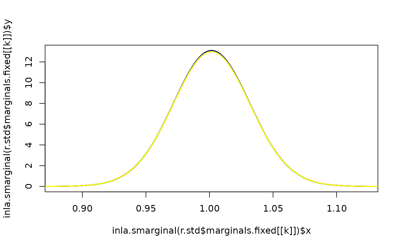
Second example

There is also another (experimental) option, that is

control.inla = list(int.stategy = "user.expert")

for which the weights $\pi(\theta_i | y)$ . The following example show how to use it, fitting the same model in three different ways.

n = 50
x = rnorm(n)
y = 1 + x + rnorm(n, sd = 0.2)
param = c(1, 0.04)
dz = 0.1
r.std = inla(y ~ 1 + x, data = data.frame(y, x),
             control.inla = list(int.strategy = "grid",
                                 dz = dz,
                                 diff.logdens = 8), 
             control.family = list(
                 hyper = list(
                     prec = list(
                         prior = "loggamma",
                         param = param))))

s = r.std$internal.summary.hyperpar[1,"sd"]
m = r.std$internal.summary.hyperpar[1,"mean"]
theta = m + s*seq(-4, 4, by = dz)
weight = dnorm(theta,  mean = m, sd = s)

r = rep(list(list()), length(theta))
for(k in seq_along(r)) {
    r[[k]] = inla(y ~ 1 + x,
                  control.family = list(
                      hyper = list(
                          prec = list(
                              initial = theta[k],
                              fixed=TRUE))),
                  data = data.frame(y, x))
}
r.merge = inla.merge(r, prob = weight)

## Warning in inla.merge(r, prob = weight): This function is experimental.

## Warning in inla.merge(r, prob = weight): Merging 'cpo' and 'pit'-results
## are/can be, approximate only

r.design = inla(y ~ 1 + x,
                data = data.frame(y, x),
                control.family = list(
                    hyper = list(
                        prec = list(
                            ## the prior here does not really matter, as we will override
                            ## it with the user.expert in any case.
                            prior = "pc.prec",
                            param = c(1, 0.01)))), 
                control.inla = list(int.strategy = "user.expert",
                                    int.design = cbind(theta, weight)))
for(k in 1:2) {
    plot(inla.smarginal(r.std$marginals.fixed[[k]]),
         lwd = 2, lty = 1, type = "l", 
         xlim = inla.qmarginal(c(0.0001, 0.9999), r.std$marginals.fixed[[k]]))
    lines(inla.smarginal(r.design$marginals.fixed[[k]]),
          lwd = 2, col = "blue", lty = 1)
    lines(inla.smarginal(r.merge$marginals.fixed[[k]]),
          lwd = 2, col = "yellow", lty = 1)
}

Haavard Rue `(hrue@r-inla.org)`

May 2017 (updated April 2019 and May 2023)

Introduction

First example

Second example

User defined integration points

Haavard Rue (hrue@r-inla.org)

May 2017 (updated April 2019 and May 2023)

Introduction

First example

Second example

Haavard Rue `(hrue@r-inla.org)`