Introduction
This is a short note to discuss the use of the new ``A-local’’ feature.
The basic issue this feature address, is that the linear predictor sometimes contains more than one element from one or more model component. For example
where is defined in and is a fixed matrix. Here, “” represents other model components in the model that are noe relevant for this discussion. Earlier, such cases have been adressed by removing the A-matrix locally and redefine it globally, by introducing for another A-matrix. The overall model, in terms of is the same.
The step with introducing is often unnecessary complicated and leads to a construction which also depends on the irrelevant parts of the model given above in “”. This can now be avoided in many cases.
First example
The general format is
Let represent the model component with elements , then the above says that
The redundancy is obvious, represents here an alternative approach to give , and we could represent the -part as as well. The for which are defined, here , is extracted from and not . If we define manually, then can be just dummy and we can move to using only. An in-between approach is also possible: Use as normal but to set (-vector), so that all information ’s influence on is from the -th row , but the information about the are taken from .
Here is a simple example with the model where is , which is simulated using
The first (traditional) approach is to use
r1 <- inla(y ~ 1 + f(i,model="iid") + f(im, copy="i"),
    family="stdnormal",
    data = data.frame(y,i,im))
The second approach is to use to define the additional contribution
A <- matrix(0,n,n)
A[row(A)-col(A) == 1] <- 1
A <- inla.as.sparse(A)
r2 <- inla(y ~ 1 + f(i, model="iid", A.local=A),
    family="stdnormal",
    data = list(y=y,i=i,A=A))
The third approach is to use with all info in the -matrix
diag(A) <- 1 ## we add also the diagonal
r3 <- inla(y ~ 1 + f(i.NA, model="iid", A.local=A, values=1:n),
    family="stdnormal",
    data = list(y=y, i.NA=rep(NA,n), A=A, n=n))
The forth approach use and also the -index to define . Note that zero-out the contribution, so in practice we only use the -matrix.
r4 <- inla(y ~ 1 + f(i, w.zero, model="iid", A.local=A),
    family="stdnormal",
    data = list(y=y, i=i, w.zero=rep(0,n), A=A, n=n))
The four approaches gives the same results
## [1] -197.1041 -197.1041 -197.1041 -197.1041The copy-approach (first element) is slightly different as it use an -copy and not an identical copy.
Example with replicate/group
A.local is replicated when and/or is used. This allows extra flexibilty.
If the dimensions of A.local do not match the dimension of , it still works. Like has length , then is normally a (sparse) matrix of size for some and . If then row are treated as empty or no A-matrix. If then only the first rows are used, with no warnings given. Here is an example where as we stack the two ’s. The result is the same as before
AA <- rbind(A,A)
r5 <- inla(y ~ 1 + f(i, w.zero, model="iid", A.local=AA),
    family="stdnormal",
    data = list(y=y, i=i, w.zero=rep(0,n), AA=AA, n=n))
r5$mlik[1,]
## log marginal-likelihood (integration)
## -197.1041Here is a somewhat more advanced example with two replicated AR1 processes.
n <- 1000
phi <- 0.9
x <- scale(arima.sim(n=n,  model = list(ar = phi)))
xx <- scale(arima.sim(n=n,  model = list(ar = phi)))
where each process is convolved with its kernel
h <- 10L
nh <- h + 1L
kern <- dnorm(-h:0, sd=h)
kern <- kern / sum(kern)
A <- inla.as.sparse(INLA:::inla.toeplitz(c(kern[nh], rep(0, n-nh), kern[1:h])))

h <- 30L
nh <- h + 1L
kern <- dnorm(-h:0, sd= h)
kern <- kern / sum(kern)
B <- inla.as.sparse(INLA:::inla.toeplitz(c(kern[nh], rep(0, n-nh), kern[1:h])))
to form the lin.predictor
Using that the second replicate is stored at indices , we can just bind and together
AB <- cbind(A, B)
r <- inla(y ~ 1 + f(idx, w, model="ar1", constr = T, A.local = AB, nrep = 2),
          data = list(y = y, idx = 1:n, AB = AB, w = rep(0, n)),
          family = "poisson")
plot(idx, eta, col="blue", lwd=2, type="l", ylim = range(pretty(eta)))
lines(idx, r$summary.linear.predictor$mean, col="red", lwd=2)
title("eta.true and E(eta|...)")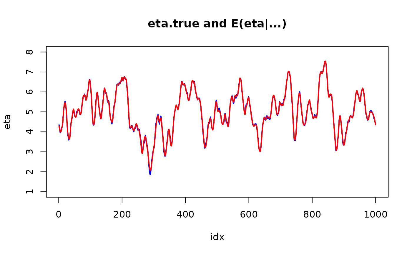
plot(idx, x, col="blue", lwd=2, type="l", ylim = range(pretty(x)))
lines(idx, r$summary.random$idx$mean[1:n], col="red", lwd=2)
title("AR1 and E(AR1|...)")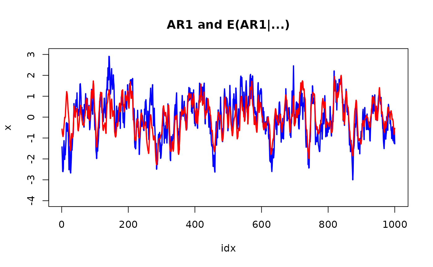
plot(idx, xx, col="blue", lwd=2, type="l", ylim = range(pretty(x)))
lines(idx, r$summary.random$idx$mean[n + 1:n], col="red", lwd=2)
title("AR1 and E(AR1|...)")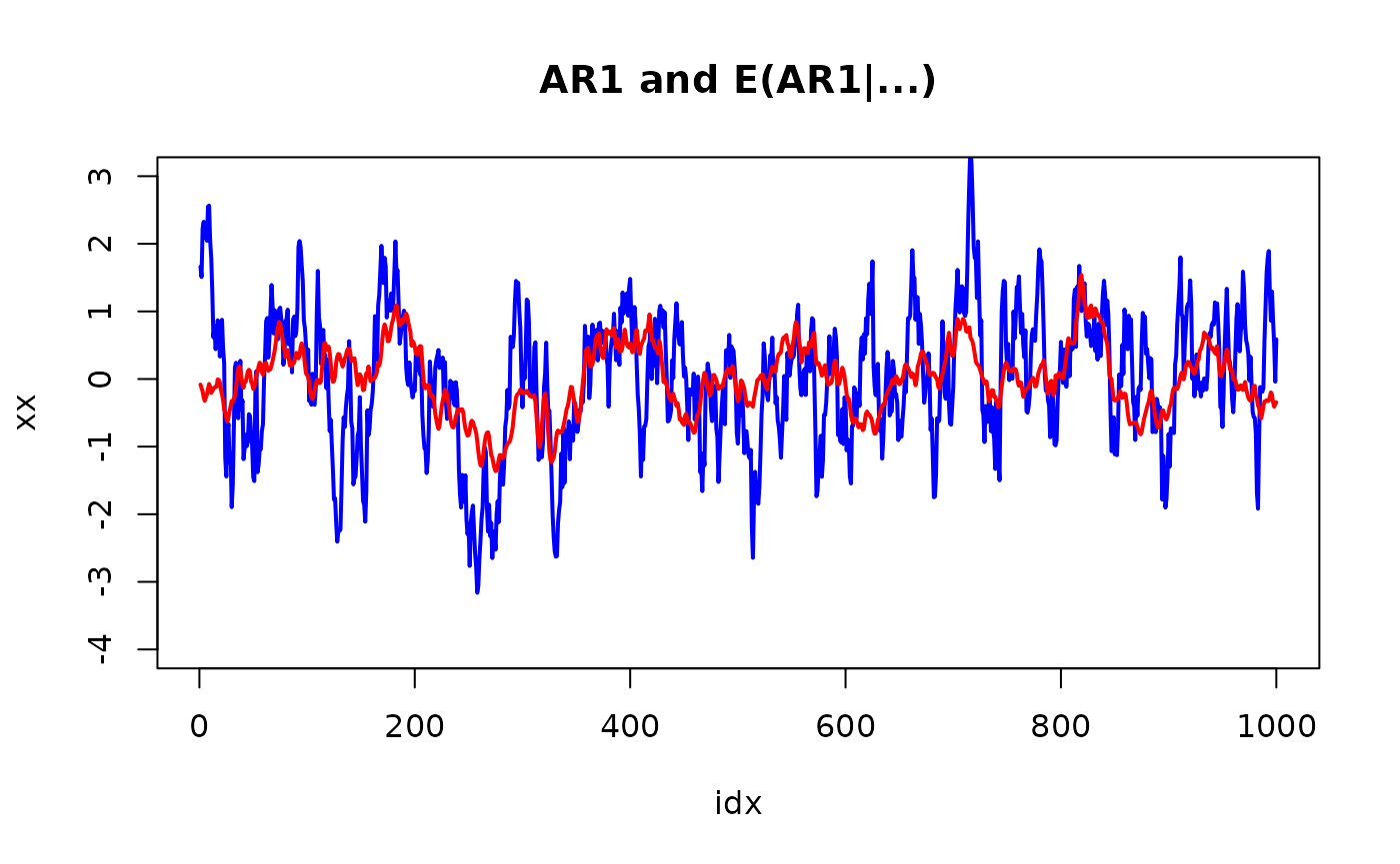
and the summary is
summary(r)## Time used:
## Pre = 0.133, Running = 6.06, Post = 0.0367, Total = 6.23
## Fixed effects:
## mean sd 0.025quant 0.5quant 0.975quant mode kld
## (Intercept) 4.998 0.003 4.991 4.998 5.005 4.998 0
##
## Random effects:
## Name Model
## idx AR1 model
##
## Model hyperparameters:
## mean sd 0.025quant 0.5quant 0.975quant mode
## Precision for idx 1.100 0.136 0.850 1.094 1.383 1.087
## Rho for idx 0.884 0.017 0.848 0.885 0.915 0.886
##
## Marginal log-Likelihood: -4500.07
## is computed
## Posterior summaries for the linear predictor and the fitted values are computed
## (Posterior marginals needs also 'control.compute=list(return.marginals.predictor=TRUE)')The z model
The new feature gives an easy way to implement the z-model, which is the classic mixed-effect model formulation
where is a fixed matrix and is zero mean Normal with precision . This is implemented in model “z” as follows.
n <- 300
m <- 30
Z <- matrix(rnorm(n*m), n, m)
rho <- 0.8
Qz <- toeplitz(rho^(0:(m-1)))
z <- inla.qsample(1, Q=Qz)
eta <- Z %*% z
s <- 0.1
y <- eta + rnorm(n, sd = s)
Using the z-model we get
r <- inla(y ~ -1 + f(idx, model="z", Z=Z, Cmatrix=Qz, precision=exp(20),
                    hyper = list(prec = list(initial = 0, fixed = TRUE))),
        data = list(y=y, idx=1:n, n=n),
        control.family = list(hyper = list(prec = list(initial = log(1/s^2), fixed= TRUE))))
Using A.local we get
rr <- inla(y ~ -1 + f(idx, model="generic", A.local=Z, Cmatrix=Qz, values=1:m,
                    hyper = list(prec = list(initial = 0, fixed = TRUE))),
        data = list(y=y, idx=rep(NA,n), n=n, m=m),
        control.family = list(hyper = list(prec = list(initial = log(1/s^2), fixed= TRUE))))
and we can compare (noting that “generic” model does not include the normalization constant wrt to the precision matrix; see the documentation)
r$mlik - (rr$mlik + 0.5 * determinant(Qz, log=TRUE)$modulus)## [,1]
## log marginal-likelihood (integration) -0.000498423
## log marginal-likelihood (Gaussian) -0.000498423## [1] 6.667828e-09## [1] 1.02281e-07Using replicate, again
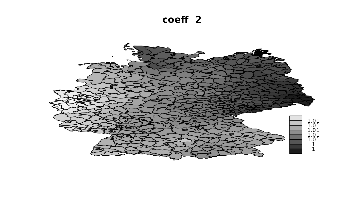
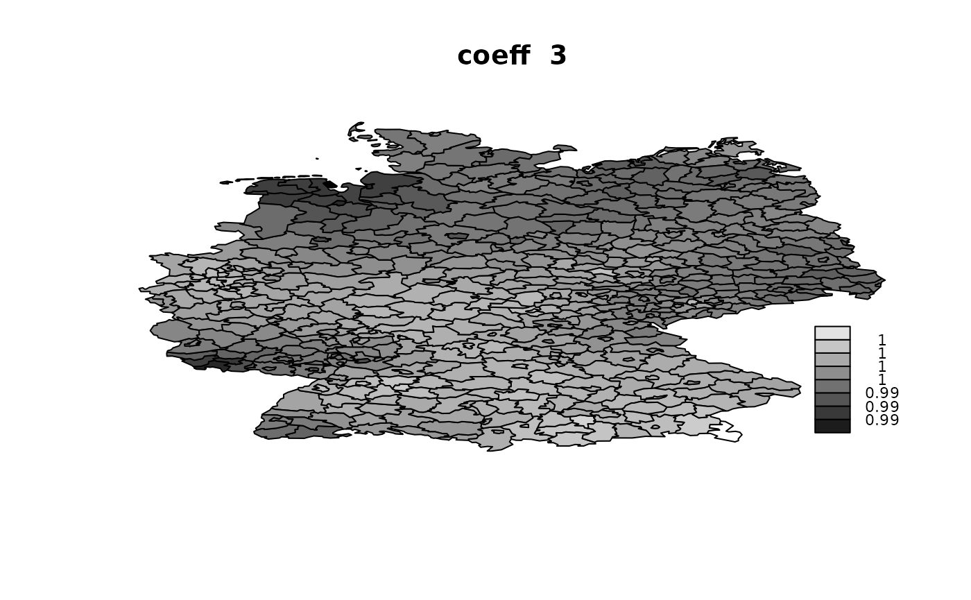
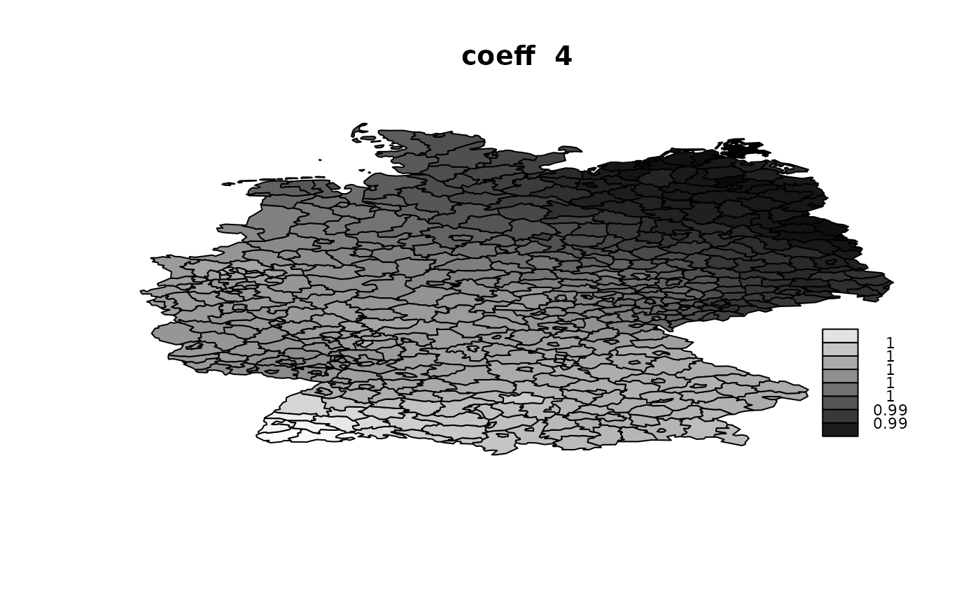
This is motivated from an example from the discussion-list, where
where the second term using a replication hence sharing the same hyperparameter. Here its written out for terms, but the aim was several terms like .
This can now be done very efficient
g <- inla.read.graph(system.file("demodata/germany.graph", package="INLA"))
source(system.file("demodata/Bym-map.R", package="INLA"))
n <- g$n
m <- 4
s <- 0.1
X <- matrix(rnorm(n*m), n, m)
y <- rowSums(X) + rnorm(n, sd = s)
A <- inla.as.sparse(diag(X[, 1]))
for(i in 2:m) {
    A <- cbind(A, inla.as.sparse(diag(X[, i])))
}

r <- inla(y ~ -1 +
              f(idx.na,
                model = "besag",
                scale.model = TRUE,
                constr = FALSE,
                nrep = m,
                graph = g,
                A.local = A,
                values = 1:n,
                hyper = list(prec = list(prior = "pc.prec",
                                         param = c(0.5, 0.01)))),
          family = "normal",
          control.family = list(hyper = list(prec = list(initial = log(1/s^2),
                                                         fixed = TRUE))),
          data = list(n = n, m = m, y = y, X = X,
idx.na = rep(NA, n)))## V1 V2 V3 V4
## Min. :1.002 Min. :0.998 Min. :0.9895 Min. :0.9862
## 1st Qu.:1.006 1st Qu.:1.004 1st Qu.:0.9945 1st Qu.:0.9912
## Median :1.007 Median :1.006 Median :0.9955 Median :0.9959
## Mean :1.007 Mean :1.006 Mean :0.9954 Mean :0.9948
## 3rd Qu.:1.008 3rd Qu.:1.008 3rd Qu.:0.9965 3rd Qu.:0.9977
## Max. :1.011 Max. :1.013 Max. :1.0001 Max. :1.0046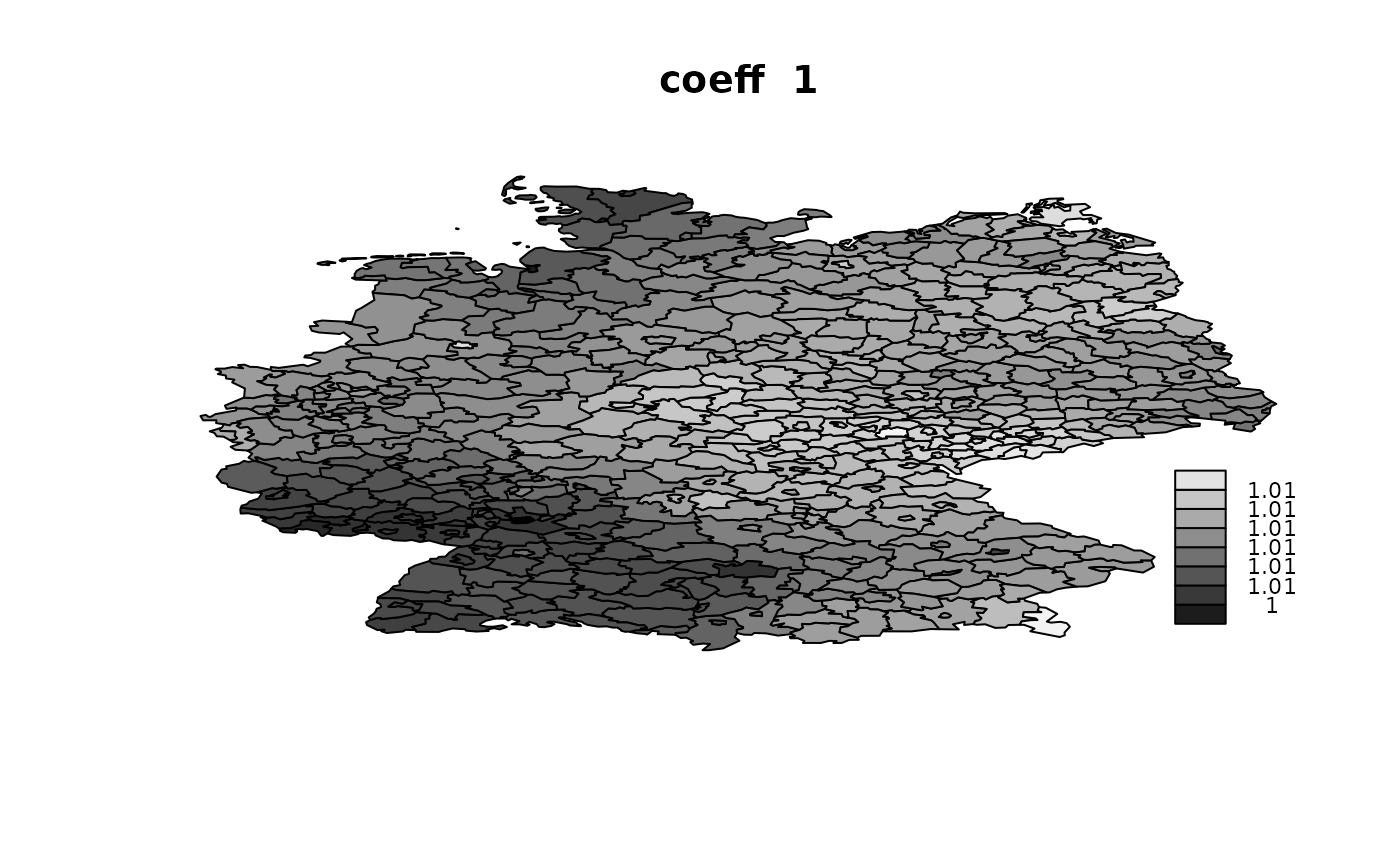
Using ‘Alocal’ in copy
This is to verify that Alocal-feature works as expected with copy. Consider this simple example
where match data as
##        y
##  [1,]  1  1
##  [2,]  2  2
##  [3,]  3  3
##  [4,]  4  4
##  [5,]  5  5
##  [6,]  6  6
##  [7,]  7  7
##  [8,]  8  8
##  [9,]  9  9
## [10,] 10 10
We can verify that this works as expected with
idx <- 1:n
iidx <- rep(NA, n)
w0 <- rep(0, n)
r <- inla(y ~ -1 +
              f(idx,
                w0,
                model = "iid",
                values = 1:n,
                hyper = list(prec = list(initial = -20,
                                         fixed = TRUE))) +
              f(iidx,
                copy = "idx",
                values = 1:n,
                A.local = A),
          data = list(idx = idx,
                      iidx = iidx,
                      w0 = w0,
                      A = A,
                      n = n),
          family = "stdnormal")
The idx part only defines the iid model, but is not
used, as the weights w0 are all zero. The distribution is
essentially uniform due to the small fixed precision.
The iidx part copy idx, and then apply
matrix A in A.local. This mean that both
idx and iidx should have mean 1, and the
-matrix
will make this fit the data.
##       [,1] [,2]
##  [1,]    1    1
##  [2,]    1    1
##  [3,]    1    1
##  [4,]    1    1
##  [5,]    1    1
##  [6,]    1    1
##  [7,]    1    1
##  [8,]    1    1
##  [9,]    1    1
## [10,] 1 1## y
## [1,] 1 1
## [2,] 2 2
## [3,] 3 3
## [4,] 4 4
## [5,] 5 5
## [6,] 6 6
## [7,] 7 7
## [8,] 8 8
## [9,] 9 9
## [10,] 10 10If we add scaling this still works
r <- inla(y ~ -1 +
              f(idx,
                w0,
                model = "iid",
                values = 1:n,
                hyper = list(prec = list(initial = -20,
                                         fixed = TRUE))) +
              f(iidx,
                copy = "idx",
                values = 1:n,
                A.local = A,
                hyper = list(beta = list(initial = 0.5))),
          data = list(idx = idx,
                      iidx = iidx,
                      w0 = w0,
                      A = A,
                      n = n),
          family = "stdnormal")
Due to the scaling, then idx has to bump to
,
but iidx is still
to fit data
##       [,1] [,2]
##  [1,]    2    1
##  [2,]    2    1
##  [3,]    2    1
##  [4,]    2    1
##  [5,]    2    1
##  [6,]    2    1
##  [7,]    2    1
##  [8,]    2    1
##  [9,]    2    1
## [10,]    2    1