Approximating joint marginals
Cristian Chiuchiolo and Haavard Rue
KAUST, Aug 2020
jmarginal.RmdIntroduction
The primary use of R-INLA is to approximate univariate
marginals of the latent field, so we can compute their marginal
summaries and densities. In applications, we sometimes need more than
this, as we are interested also in statistics which involve more several
of the components of the latent field, and/or, a joint posterior
approximation to a subset of the latent field.
The way around this issue, have earlier resolved to stochastic
simulation, using the function inla.posterior.sample. This
function samples from joint approximation to the full posterior which
INLA construct, but do so for the whole latent field. Using
these samples, we can compute the density of the relevant statistics
and/or use standard methods to represent a joint marginal.
This vignette introduces a new tool which computes a deterministic
approximation to the joint marginal for a subset of the latent field
using R-INLA. This approximation is explicitly available,
and constructed using skew-normal marginals and a Gaussian copula, hence
restricted to a joint approximation of a modest dimension.
The key specification is using an argument selection in
the inla()-call, which defines the subset, and then the
joint marginal approximation is made available in
result$selection.
Note that when using the classic-mode, like
inla.setOption(inla.mode="classic")then linear predictors can also be used. With the default
inla.setOption(inla.mode="compact")then the linear predictor can not be used as it is not explicitly part of the latent model.
Theory reference
For any with data and set of parameters with being the latent field and the hyperparameters, the resulting joint posterior approximation is stated as
where
is the Gaussian approximation. This expression recalls a Gaussian
mixture distribution with weights
obtained in the grid
exploration of the hyperparameter posterior marginals. For more
insights, we suggest checking sources like Rue,
Martino, and Chopin (2009), Martins et al.
(2013), Blangiardo et al. (2013),
or the recent review by Martino and Riebler
(2019). The Gaussian approximation used in is both mean and
skewness corrected since it exploits Skew-Normal marginals of the latent
field into a Gaussian copula structure (see Ferkingstad and Rue (2015) for details). These
corrections are available in inla.posterior.sample as
First example
We will illustrate this new feature using a simple example.
n = 100
x = rnorm(n, mean = 1, sd = 0.3)
xx = rnorm(n, mean = -2, sd = 0.3)
y = rpois(n, lambda = exp(x + xx))
r = inla(y ~ 1 + x + xx,
         data = data.frame(y, x, xx),
         family = "poisson")
Let us compute the joint marginal for the effect of x,
xx and the intercept. This is specified using the argument
selection, which is a named list of indices to select.
Names are those given the formula, plus standard names like
(Intercept), Predictor and
APredictor. So that
selection = list(Predictor = 3:4, x = 1, xx = 1)say that we want the joint marginal for the
and
element of Predictor and the first element of
x and xx. (Well, x and
xx only have one element, so then there is not else we can
do in this case.)
If we pass selection, then we have to rerun
inla() in classic-mode, as Predictor in the selection is
not supported in compact-mode.
rs = inla(y ~ 1 + x + xx,
          data = data.frame(y, x, xx),
          family = "poisson",
          inla.mode = "classic",
          control.compute = list(return.marginals.predictor = TRUE),
          control.predictor = list(compute = TRUE),
          selection = selection)
We obtain
#summary(rs$selection)
print(rs$selection)
$names
[1] "Predictor:3" "Predictor:4" "x:1" "xx:1"
$mean
[1] -0.7122299 -1.5151313 1.6615111 1.9552106
$cov.matrix
[,1] [,2] [,3] [,4]
[1,] 0.08282108 0.02406951 0.13371942 -0.03139152
[2,] 0.02406951 0.05740996 -0.06885452 -0.08589163
[3,] 0.13371942 -0.06885452 0.44694651 0.10015771
[4,] -0.03139152 -0.08589163 0.10015771 0.32337255
$skewness
[1] -0.245851347 -0.268814049 -0.001085065 -0.025390461
$marginal.sn.par
$marginal.sn.par$xi
[1] -0.473225 -1.310130 1.752585 2.176786
$marginal.sn.par$omega
[1] 0.3740915 0.3153339 0.6747154 0.6103016
$marginal.sn.par$alpha
[1] -1.3367458 -1.4054017 -0.1716471 -0.5109904The Gaussian copula is given by the mean and the
cov.matrix objects, while the Skew-Normal marginals are
given implicitly using the marginal mean and variance in the Gaussian
copula and the listed skewness. Moreover the respective Skew-Normal
mapping parameters for the marginals
are provided in the object ‘marginal.sn.par’. The names are
given as a separate entry instead of naming each individual result, to
save some storage.
There are utility functions to sample and evaluate samples from this
joint marginal, similar to inla.posterior.sample and
inla.posterior.sample.eval.
ns = 10000
xs = inla.rjmarginal(ns, rs) ## or rs$selection
str(xs)
List of 2
$ samples : num [1:4, 1:10000] -1.084 -1.5174 0.8702 1.9861 0.0667 ...
..- attr(*, "dimnames")=List of 2
.. ..$ : chr [1:4] "Predictor:3" "Predictor:4" "x:1" "xx:1"
.. ..$ : chr [1:10000] "sample:1" "sample:2" "sample:3" "sample:4" ...
$ log.density: Named num [1:10000] 4.64 -2.31 4.38 4.62 4.81 ...
..- attr(*, "names")= chr [1:10000] "sample:1" "sample:2" "sample:3" "sample:4" ...whose output is a matrix where each row contains the samples for the variable in each column
 We can compare the approximation of
 Predictor:3 to the one
computed by the inla() call,
hist(xs$samples["Predictor:3",], n = 300, prob = TRUE,
main = 'Histogram of Predictor:3', xlab = 'Samples
from the joint and linear predictor marginal (black straight line)')
lines(inla.smarginal(rs$marginals.linear.predictor[[3]]), lwd = 3)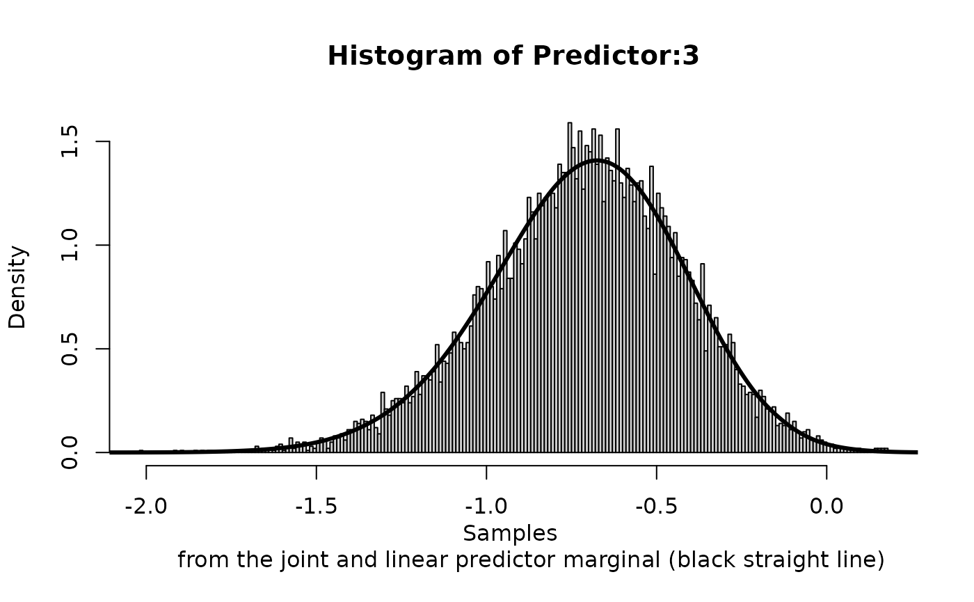 These marginals are not exactly the same (as they are different
approximations), but should be very similar.
These marginals are not exactly the same (as they are different
approximations), but should be very similar.
Deterministic Joint approximation
As a conclusion to this vignette we show an additional joint posterior related tool. The following INLA function computes a deterministic approximation for the joint posterior sampler and must be considered experimental. The function is strictly related to the selection type INLA setting. Deterministic posterior marginals for the previous example can be obtained as follows
dxs = inla.1djmarginal(jmarginal = rs$selection)
str(dxs)
List of 4
$ Predictor:3: num [1:63, 1:2] -2.46 -2.3 -2.13 -1.93 -1.78 ...
..- attr(*, "dimnames")=List of 2
.. ..$ : NULL
.. ..$ : chr [1:2] "x" "y"
$ Predictor:4: num [1:63, 1:2] -2.99 -2.85 -2.7 -2.54 -2.41 ...
..- attr(*, "dimnames")=List of 2
.. ..$ : NULL
.. ..$ : chr [1:2] "x" "y"
$ x:1 : num [1:63, 1:2] -1.818 -1.519 -1.192 -0.826 -0.54 ...
..- attr(*, "dimnames")=List of 2
.. ..$ : NULL
.. ..$ : chr [1:2] "x" "y"
$ xx:1 : num [1:63, 1:2] -1.0736 -0.8079 -0.5178 -0.1949 0.0573 ...
..- attr(*, "dimnames")=List of 2
.. ..$ : NULL
.. ..$ : chr [1:2] "x" "y"The output is a list with all computed marginals and a matrix summary output in INLA style. Marginal can be accessed and plotted by using the respective names in the selection
ggplot(data = data.frame(y = xs$samples["Predictor:3",]), aes(y, after_stat(density), colour = "True")) +
  stat_density(alpha = .1) +
  geom_line(data = as.data.frame(dxs$`Predictor:3`), aes(x = x, y = y, colour = "Deterministic"))+
  labs(title= '"Marginal Results for Predictor:3"', x='x', y='Density') +
  scale_colour_manual("",
                      breaks = c("True", "Deterministic"),
values = c("black", "red")) 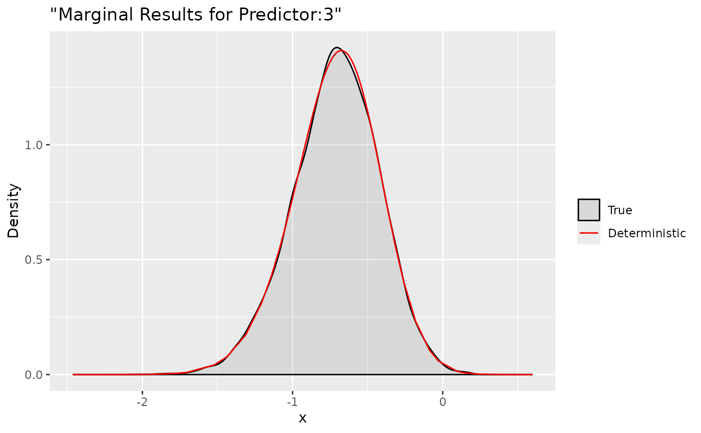
ggplot(data = data.frame(y = xs$samples["Predictor:4",]), aes(y, after_stat(density), colour = "True")) +
  stat_density(alpha = .1) +
  geom_line(data = as.data.frame(dxs$`Predictor:4`), aes(x = x, y = y, colour = "Deterministic"))+
  labs(title= '"Marginal Results for Predictor:4"', x='x', y='Density') +
  scale_colour_manual("",
                      breaks = c("True", "Deterministic"),
values = c("black", "red")) 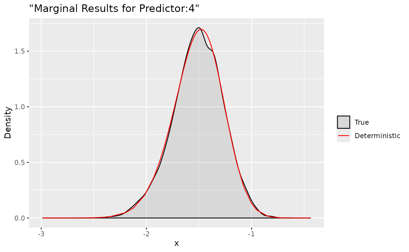
ggplot(data = data.frame(y = xs$samples["x:1",]), aes(y, after_stat(density), colour = "True")) +
  stat_density(alpha = .1) +
  geom_line(data = as.data.frame(dxs$`x:1`), aes(x = x, y = y, colour = "Deterministic"))+
  labs(title= '"Marginal Results for x:1"', x='x', y='Density') +
  scale_colour_manual("",
                      breaks = c("True", "Deterministic"),
values = c("black", "red")) 
ggplot(data = data.frame(y = xs$samples["xx:1",]), aes(y, after_stat(density), colour = "True")) +
  stat_density(alpha = .1) +
  geom_line(data = as.data.frame(dxs$`xx:1`), aes(x = x, y = y, colour = "Deterministic"))+
  labs(title= '"Marginal Results for xx:1"', x='x', y='Density') +
  scale_colour_manual("",
                      breaks = c("True", "Deterministic"),
values = c("black", "red")) 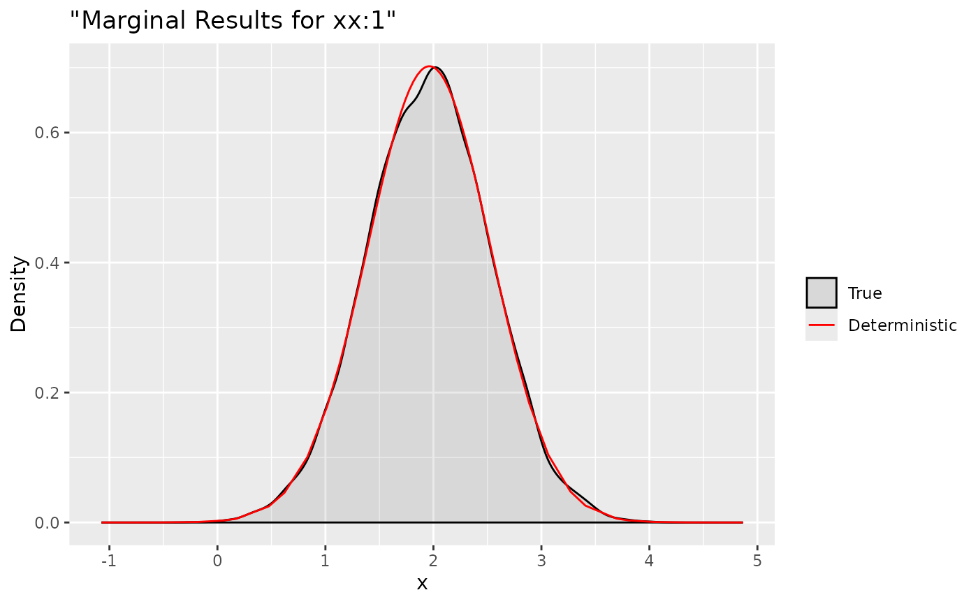
Here we compare the deterministic marginals with their sampling
version. They are quite accurate and can provide more informations.
Indeed, a complete summary based on these deterministic results is
achievable with a personalized summary function
summary(rs$selection)[1] "Joint marginal is computed for: "
mean sd 0.025quant 0.5quant 0.975quant mode
Predictor:3 -0.7122299 0.2877865 -1.3116414 -0.6999187 -0.1811392 -0.674685
Predictor:4 -1.5151313 0.2396038 -2.0168857 -1.5038653 -1.0756582 -1.480695
x:1 1.6615111 0.6685406 0.3508477 1.6616320 2.9714875 1.661867
xx:1 1.9552106 0.5686586 0.8335793 1.9576236 3.0631404 1.962457where posterior estimates and quantiles are computed for all the
selected marginals. Along the same line, we can easily compute multiple
deterministic linear combinations through the function
inla.tjmarginaland a matrix object A with the respective
indexes
      [,1] [,2] [,3] [,4]
Test1    1    1    0    0
Test2    0    0    1    1
We define two linear combinations:
Predictor:3+Predictor:4 and x:1+xx:1
respectively. Then we can use the cited function which has the same
class of selection object
m = inla.tjmarginal(jmarginal = rs, A = A)
m
class(m)
$names
[1] "Test1" "Test2"
$mean
[,1]
Test1 -2.227361
Test2 3.616722
$cov.matrix
Test1 Test2
Test1 0.18837006 -0.05241825
Test2 -0.05241825 0.97063448
$skewness
[1] -0.116903541 -0.005221538
$marginal.sn.par
$marginal.sn.par$xi
Test1 Test2
-1.946024 3.843311
$marginal.sn.par$omega
Test1 Test2
0.5172241 1.0109289
$marginal.sn.par$alpha
[1] -0.9318140 -0.2927042
[1] "inla.jmarginal"
dxs.lin = inla.1djmarginal(jmarginal = m)
str(dxs.lin)

fun1 <- function(...) {Predictor[1]+Predictor[2]}
fun2 <- function(...) {x+xx}

xs.lin1 = inla.rjmarginal.eval(fun1, xs)
xs.lin2 = inla.rjmarginal.eval(fun2, xs)

ggplot(data = data.frame(y = xs.lin1[1, ]), aes(y, after_stat(density), colour = "True")) +
  stat_density(alpha = .1) +
  geom_line(data = as.data.frame(dxs.lin$Test1), aes(x = x, y = y, colour = "Deterministic"))+
  labs(title= '"Marginal Results for Lin1"', x='x', y='Density') +
  scale_colour_manual("",
                      breaks = c("True", "Deterministic"),
values = c("black", "red")) 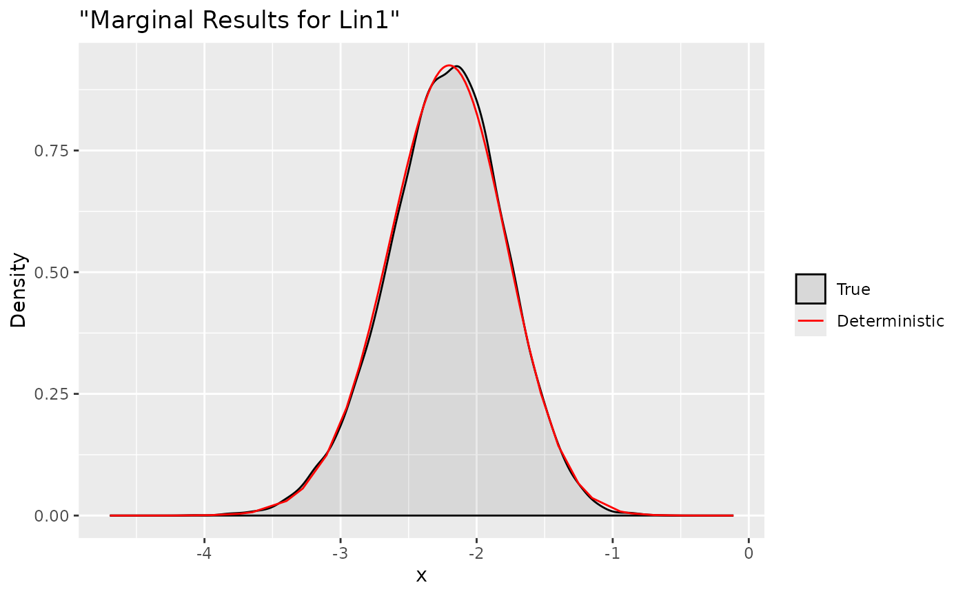
ggplot(data = data.frame(y = xs.lin2[1, ]), aes(y, after_stat(density), colour = "True")) +
  stat_density(alpha = .1) +
  geom_line(data = as.data.frame(dxs.lin$Test2), aes(x = x, y = y, colour = "Deterministic"))+
  labs(title= '"Marginal Results for Lin2"', x='x', y='Density') +
  scale_colour_manual("",
                      breaks = c("True", "Deterministic"),
values = c("black", "red")) 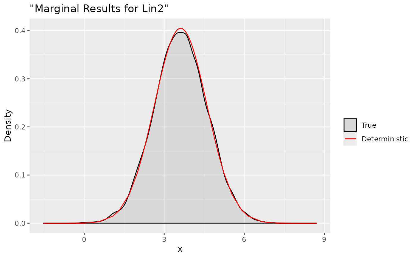
List of 2
 $ Test1: num [1:63, 1:2] -4.69 -4.48 -4.23 -3.96 -3.75 ...
  ..- attr(*, "dimnames")=List of 2
  .. ..$ : NULL
  .. ..$ : chr [1:2] "x" "y"
 $ Test2: num [1:63, 1:2] -1.5314 -1.0875 -0.6017 -0.0595 0.3657 ...
  ..- attr(*, "dimnames")=List of 2
  .. ..$ : NULL
  .. ..$ : chr [1:2] "x" "y"
and accomplish the job with summaries
summary(m)[1] "Joint marginal is computed for: "
mean sd 0.025quant 0.5quant 0.975quant mode
Test1 -2.227361 0.4340162 -3.103352 -2.218761 -1.399908 -2.201414
Test2 3.616722 0.9852078 1.683261 3.617580 5.545308 3.619285Transformations of the marginal terms or linear combinations are
possible as well. We just need to use inla.tmarginal as
follows
fun.exp <- function(x) exp(x)

fun5 <- function(...) {exp(x)}
fun6 <- function(...) {exp(xx)}
fun7 <- function(...) {exp(x+xx)}

tdx <- inla.tmarginal(fun = fun.exp, marginal = dxs$`x:1`)
tdxx <- inla.tmarginal(fun = fun.exp, marginal = dxs$`xx:1`)
tdx.lin <- inla.tmarginal(fun = fun.exp, marginal = dxs.lin$Test2)

tx = inla.rjmarginal.eval(fun5, xs)
txx = inla.rjmarginal.eval(fun6, xs)
tx.lin = inla.rjmarginal.eval(fun7, xs)

ggplot(data = data.frame(y = tx[1, ]), aes(y, after_stat(density), colour = "True")) +
  stat_density(alpha = .1) +
  geom_line(data = as.data.frame(tdx), aes(x = x, y = y, colour = "Deterministic"))+
  labs(title= '"Marginal Results for exp(x:1)"', x='x', y='Density') +
  scale_colour_manual("",
                      breaks = c("True", "Deterministic"),
values = c("black", "red")) 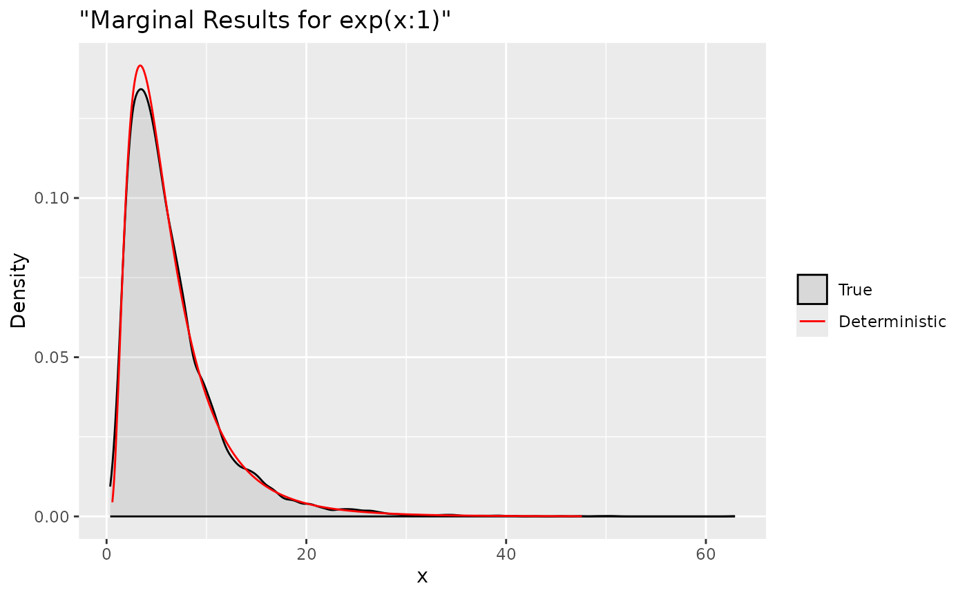
ggplot(data = data.frame(y = txx[1, ]), aes(y, after_stat(density), colour = "True")) +
  stat_density(alpha = .1) +
  geom_line(data = as.data.frame(tdxx), aes(x = x, y = y, colour = "Deterministic"))+
  labs(title= '"Marginal Results for exp(xx:1)"', x='x', y='Density') +
  scale_colour_manual("",
                      breaks = c("True", "Deterministic"),
values = c("black", "red")) 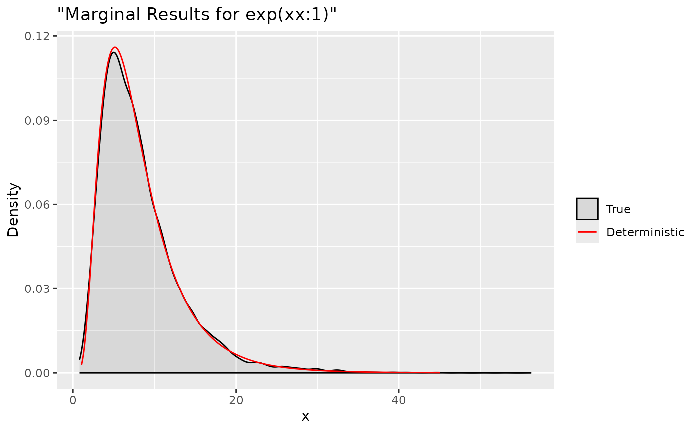
ggplot(data = data.frame(y = tx.lin[1, ]), aes(y, after_stat(density), colour = "True")) +
  stat_density(alpha = .1) +
  geom_line(data = as.data.frame(tdx.lin), aes(x = x, y = y, colour = "Deterministic"))+
  labs(title= '"Marginal Results for exp(x:1+xx:1)"', x='x', y='Density') +
  scale_colour_manual("",
                      breaks = c("True", "Deterministic"),
values = c("black", "red")) 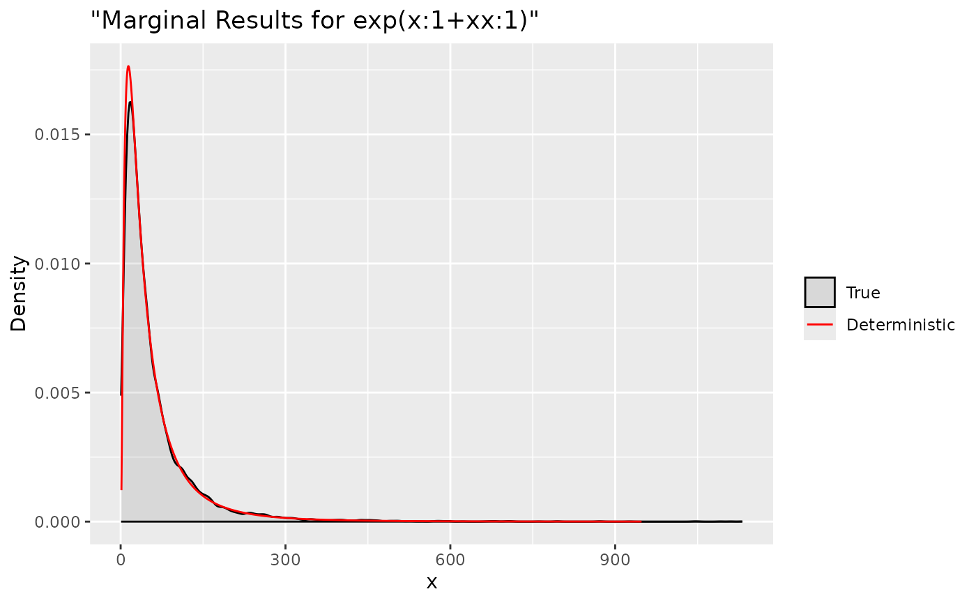
Summaries for all marginal transformations can be obtained through
inla.zmarginal
expx = inla.zmarginal(marginal = tdx, silent = TRUE)
expxx = inla.zmarginal(marginal = tdxx, silent = TRUE)
expx.lin = inla.zmarginal(marginal = tdx.lin, silent = TRUE)

exp.summaries = rbind(expx, expxx, expx.lin)
exp.summaries
mean sd quant0.025 quant0.25 quant0.5 quant0.75 quant0.975
expx 6.562767 4.800732 1.416448 3.34579 5.256162 8.252482 19.39278
expxx 8.279929 4.985013 2.301916 4.813455 7.071526 10.36358 21.27648
expx.lin 59.8277 71.62403 5.17904 18.93143 37.00421 72.05418 253.5345