Estimate posterior distributions of fitted lambda values

For use with 'nmix' and 'nmixnb' models. This function takes the information contained in an object returned by inla() and uses the contents to create fitted lambda values using the linear predictor for log(lambda), the input covariate values, and samples from the posteriors of the model hyperparameters. Fitted values from the linear predictor are exponentiated, by default, before being returned.

inla.nmix.lambda.fitted(
  result,
  sample.size = 1000,
  return.posteriors = FALSE,
  scale = "exp"
)

Arguments

result: The output object from a call to inla(), where the family argument has been set to 'nmix' or 'nmixnb'. For the function to work, the call to inla() should also include the argument control.compute=list(config = TRUE)).
sample.size: The size of the sample from the posteriors of the model hyperparameters. This sample size ends up being the size of the estimated posterior for a fitted lambda value. Default is 1000. Larger values are recommended.
return.posteriors: A logical value for whether or not to return the full estimated posteriors for each fitted value (TRUE), or just a summary of the posteriors (FALSE). Default is FALSE.
scale: A character string, where the default string, "exp", causes values from the linear predictor to be exponentiated before being returned. The string, "log", causes values to be returned on the log(lambda) scale.

Value

fitted.summary: A data frame with summaries of estimated posteriors of fitted lambda values. The number of rows equals the number of rows in the data used to create the 'nmix' or 'nmixnb' model. There are six columns of summary statistics for each estimated posterior. Columns include an index, mean.lambda, sd.lambda, quant025.lambda, median.lambda, quant975.lambda, and mode.lambda.
fitted.posteriors: A data frame containing samples that comprise the full estimated posteriors of fitted values. The number of rows equals the number of rows in the data used to create the 'nmix' or 'nmixnb' model. The number of columns equals one plus the number of samples specified by the sample.size argument.

Note

This function is experimental.

References

See documentation for families "nmix" and "nmixmb": inla.doc("nmix")

Author

Tim Meehan tmeehan@audubon.org

Examples


## an example analysis of an N-mixture model using simulated data
## set parameters
n <- 75                       # number of study sites
nrep.max <- 5                 # number of surveys per site
b0 <- 0.5                     # lambda intercept, expected abundance
b1 <- 2.0                     # effect of x1 on lambda
a0 <- 1.0                     # p intercept, detection probability
a2 <- 0.5                     # effect of x2 on p
size <- 3.0                   # size of theta
overdispersion <- 1 / size    # for negative binomial distribution

## make empty vectors and matrix
x1 <- c(); x2 <- c()
lambdas <- c(); Ns <- c()
y <- matrix(NA, n, nrep.max)

## fill vectors and matrix
for(i in 1:n) {
    x1.i <- runif(1) - 0.5
    lambda <- exp(b0 + b1 * x1.i)
    N <- rnbinom(1, mu = lambda, size = size)
    x2.i <- runif(1) - 0.5
    eta <- a0 + a2 * x2.i
    p <- exp(eta) / (exp(eta) + 1)
    nr <- sample(1:nrep.max, 1)
    y[i, 1:nr] <- rbinom(nr, size = N, prob = p)
    x1 <- c(x1, x1.i); x2 <- c(x2, x2.i)
    lambdas <- c(lambdas, lambda); Ns <- c(Ns, N)
}

## bundle counts, lambda intercept, and lambda covariates
Y <- inla.mdata(y, 1, x1)

## run inla and summarize output
result <- inla(Y ~ 1 + x2,
  data = list(Y=Y, x2=x2),
  family = "nmixnb",
  control.fixed = list(mean = 0, mean.intercept = 0, prec = 0.01,
                      prec.intercept = 0.01),
  control.family = list(hyper = list(theta1 = list(param = c(0, 0.01)),
                                    theta2 = list(param = c(0, 0.01)),
                                    theta3 = list(prior = "flat",
                                                 param = numeric()))),
  control.compute=list(config = TRUE)) # important argument
#> 
#>  *** inla.core.safe:  The inla program failed, but will rerun in case better initial values may help. try=1/1 
#> 
#>  *** inla.core.safe:  rerun with improved initial values 
summary(result)
#> Time used:
#>     Pre = 0.175, Running = 0.244, Post = 0.0385, Total = 0.457 
#> Fixed effects:
#>               mean    sd 0.025quant 0.5quant 0.975quant   mode kld
#> (Intercept)  0.616 0.209      0.188    0.622      1.009  0.622   0
#> x2          -0.226 0.601     -1.416   -0.222      0.947 -0.223   0
#> 
#> Model hyperparameters:
#>                                         mean    sd 0.025quant 0.5quant
#> beta[1] for NMixNB observations        0.390 0.145      0.104    0.390
#> beta[2] for NMixNB observations        2.107 0.468      1.203    2.102
#> overdispersion for NMixNB observations 0.427 0.215      0.134    0.385
#>                                        0.975quant  mode
#> beta[1] for NMixNB observations             0.675 0.390
#> beta[2] for NMixNB observations             3.046 2.077
#> overdispersion for NMixNB observations      0.959 0.306
#> 
#> Marginal log-Likelihood:  -221.93 
#>  is computed 
#> Posterior summaries for the linear predictor and the fitted values are computed
#> (Posterior marginals needs also 'control.compute=list(return.marginals.predictor=TRUE)')
#> 

## get and evaluate fitted values
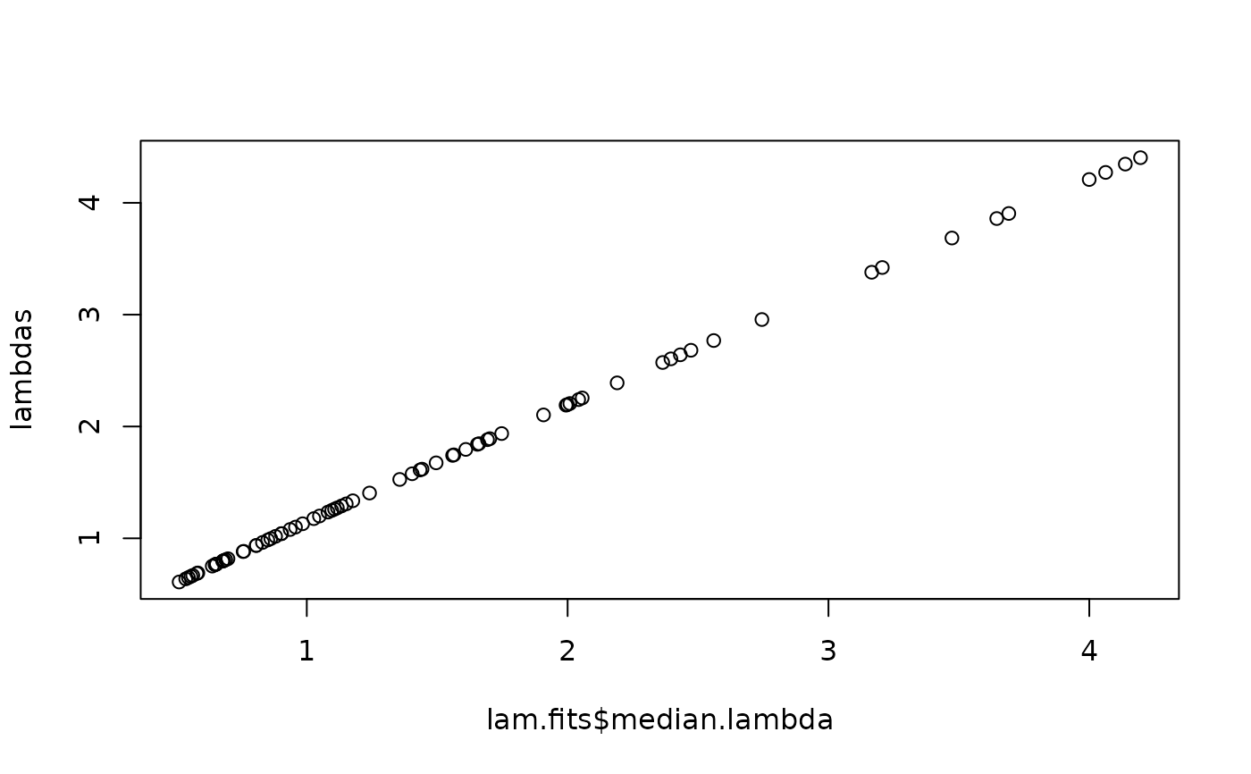
lam.fits <- inla.nmix.lambda.fitted(result, 5000)$fitted.summary
plot(lam.fits$median.lambda, lambdas)

round(sum(lam.fits$median.lambda), 0); sum(Ns)
#> [1] 116
#> [1] 117