Proper scoring rules for Bayesian model comparison

inlabru practitioners often evaluate models by how well their posterior predictive distribution covers held-out data, rather than by point-forecast error alone. A scoring rule is proper if it is minimised in expectation only when the forecaster reports their true predictive distribution — this rules out gaming by sharpening or widening predictions artificially.

inlaops provides bru_score() to compute four scores using the full posterior predictive distribution via inlabru::generate() and the scoringRules package. CRPS and log-score are strictly proper. Squared error evaluates only the posterior mean. Dawid-Sebastiani is proper for location-scale families.

Setup

library(inlabru)
library(inlaops)
library(scoringRules)
library(broom)
library(dplyr)
library(ggplot2)

The four scores

Score	Formula	Interpretation
CRPS	$\text{E}[\\|X - y\\|] - \frac{1}{2}\text{E}[\\|X - X'\\|]$	Lower is better. Generalises MAE. Works for any distribution.
Log-score	$-\log p(y)$	Lower is better. Penalises overconfident wrong predictions heavily.
SE	$(y - \hat{\mu})^2$	Squared error of the posterior mean.
Dawid-Sebastiani	$\frac{(y - \hat{\mu})^2}{\hat{\sigma}^2} + \log \hat{\sigma}^2$	Penalises miscalibrated variance.

CRPS and log-score are fully proper — they evaluate the entire predictive distribution, not just the mean or variance. SE only assesses the posterior mean and ignores predictive uncertainty. Dawid-Sebastiani is a Gaussian approximation to the log-score.

Example: comparing two models

set.seed(42)
n   <- 500
dat <- data.frame(
  x1 = rnorm(n),
  x2 = rnorm(n),
  x3 = rnorm(n)
)
dat$y <- 1.5 + 0.9 * dat$x1 + 0.3 * dat$x2 + rnorm(n, sd = 0.8)

# Hold out 20% for evaluation
idx_holdout <- sample(n, size = 100L)
train_dat   <- dat[-idx_holdout, ]
test_dat    <- dat[ idx_holdout, ]

Fit two models: a correctly-specified model and a model that omits x2.

fit_full <- bru(
  y ~ Intercept(1) + x1 + x2,
  family  = "gaussian",
  data    = train_dat,
  options = bru_options(control.compute = list(config = TRUE, dic = TRUE, waic = TRUE))
)

fit_reduced <- bru(
  y ~ Intercept(1) + x1,
  family  = "gaussian",
  data    = train_dat,
  options = bru_options(control.compute = list(config = TRUE, dic = TRUE, waic = TRUE))
)

Score both models against the holdout set. bru_score() calls inlabru::generate() to draw raw posterior samples and passes them to scoringRules.

The prediction formula must produce samples of Y, including the observation-model stochasticity. The package is family-agnostic — you write the appropriate r*() call yourself. Inside an inlabru::generate() formula the predictor is evaluated once per posterior sample: latent-field symbols (Intercept, field, …) are scalars per sample, and covariates (x1, x2) are vectors over observations. So length(<covariate>) is the per-sample observation count for the r*() call:

For continuous families the observation noise is a hyperparameter. Hyperparameters are available inside the formula under their standardised names (see inlabru::bru_standardise_names()), so the Gaussian SD is sampled jointly with the latent field:

scores_full <- bru_score(
  fit_full,
  newdata      = test_dat,
  pred_formula = ~ rnorm(
    length(x1), mean = Intercept + x1 + x2,
    sd   = 1 / sqrt(Precision_for_the_Gaussian_observations)
  ),
  y_col        = "y",
  n_samples    = 2000L,
  seed         = 1L
)

scores_reduced <- bru_score(
  fit_reduced,
  newdata      = test_dat,
  pred_formula = ~ rnorm(
    length(x1), mean = Intercept + x1,
    sd   = 1 / sqrt(Precision_for_the_Gaussian_observations)
  ),
  y_col        = "y",
  n_samples    = 2000L,
  seed         = 1L
)

rownames(fit_full$summary.hyperpar) lists the hyperparameters; pass them through inlabru::bru_standardise_names() to get the formula names.

Dropping the rnorm(...) layer would make bru_score() compute CRPS and log-score against draws of the posterior mean — understating predictive variance and yielding optimistic scores.

Summarise mean scores across holdout observations:

bind_rows(
  mutate(scores_full,    model = "full"),
  mutate(scores_reduced, model = "reduced")
) |>
  group_by(model) |>
  summarise(
    mean_crps = mean(crps),
    mean_logs = mean(logs),
    mean_rmse = sqrt(mean(se))
  )
#> # A tibble: 2 × 4
#>   model   mean_crps mean_logs mean_rmse
#>   <chr>       <dbl>     <dbl>     <dbl>
#> 1 full        0.447      1.18     0.786
#> 2 reduced     0.452      1.21     0.796

The full model scores better on all three metrics.

Visualising score distributions

Mean scores can hide important heterogeneity. Plot the per-observation score distributions to identify systematic patterns:

bind_rows(
  mutate(scores_full,    model = "full"),
  mutate(scores_reduced, model = "reduced")
) |>
  ggplot(aes(x = crps, fill = model)) +
  geom_density(alpha = 0.5) +
  labs(x = "CRPS (lower is better)", y = "Density") +
  theme_minimal()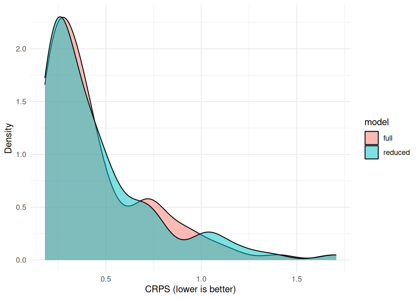

Observations where the reduced model scores much worse than the full model are precisely those with large x2 values — confirming that omitting x2 hurts predictions at the tails.

Relationship to WAIC and DIC

WAIC and DIC are information criteria computed on the training data. Proper scoring rules are computed against genuinely held-out observations.

Metric	Computed on	Accounts for overfitting?	Available at serving time?
DIC	Training	Via effective parameters	No — pin metadata only
WAIC	Training	More reliably than DIC	No — pin metadata only
CRPS / log-score	Holdout	Yes	Via `bru_score()`

Use WAIC/DIC for fast model selection during development (no holdout needed). Use CRPS/log-score for final model comparison and reporting. WAIC and DIC come from glance(), provided by inlabru:

glance(fit_full)
#> # A tibble: 1 × 5
#>     dic  waic marginal_loglik  nobs elapsed
#>   <dbl> <dbl>           <dbl> <int>   <dbl>
#> 1  973.  973.           -513.   400   0.641

Scoring spatial and non-Gaussian models

The contract is the same for spatial and non-spatial fits: pred_formula must produce samples of Y. The package does not inject family-aware observation noise — write the appropriate r*() call.

The blocks below are illustrative API sketches, not runnable end-to-end (they reference spatial_fit, poisson_fit, etc. — substitute your own fitted model). They show the formula shape per family:

# Spatial Gaussian model with SPDE field
spatial_scores <- bru_score(
  spatial_fit,
  newdata      = holdout_sp,              # SpatialPointsDataFrame or sf
  pred_formula = ~ rnorm(
    length(x1), mean = Intercept + field,
    sd   = 1 / sqrt(Precision_for_the_Gaussian_observations)
  ),
  y_col        = "y",
  n_samples    = 1000L
)

# Poisson — write the rpois yourself.
poisson_scores <- bru_score(
  poisson_fit,
  newdata      = holdout_sp,
  pred_formula = ~ rpois(length(x1), exp(Intercept + field)),
  y_col        = "counts",
  n_samples    = 1000L
)

# Binomial — pass the trial count via newdata column (e.g. `trials`).
# Inside the formula, covariate columns are vectors so `trials` and
# `length(trials)` both work.
binomial_scores <- bru_score(
  binomial_fit,
  newdata      = holdout_sp,
  pred_formula = ~ rbinom(
    length(trials), size = trials,
    prob = plogis(Intercept + field)
  ),
  y_col        = "successes",
  n_samples    = 1000L
)

# Negative binomial — INLA's nbinomial parameterisation uses size on the
# precision scale; check your fit's hyperparameter names. A simpler path
# when you don't want to bake INLA's hyperpar names into the formula is
# to score on a known approximate dispersion:
nb_scores <- bru_score(
  nb_fit,
  newdata      = holdout_sp,
  pred_formula = ~ rnbinom(
    length(x1), mu = exp(Intercept + field),
    size = known_size
  ),
  y_col        = "counts",
  n_samples    = 1000L
)

For zero-inflated families, sample the mixture explicitly: ifelse(runif(length(x), ...) < pi, 0, rpois(length(x), lambda)).

Notes on `n_samples`

bru_score() uses inlabru::generate() which draws from the full joint posterior via inla.posterior.sample(). Increasing n_samples reduces Monte Carlo variance in the scores at the cost of computation time.

For development and model comparison: 500–1000 samples is usually sufficient.
For final evaluation and reporting: 2000–5000 samples.
CRPS converges faster than log-score, which requires accurate tail probability estimates.