Plot a bayesOpt object

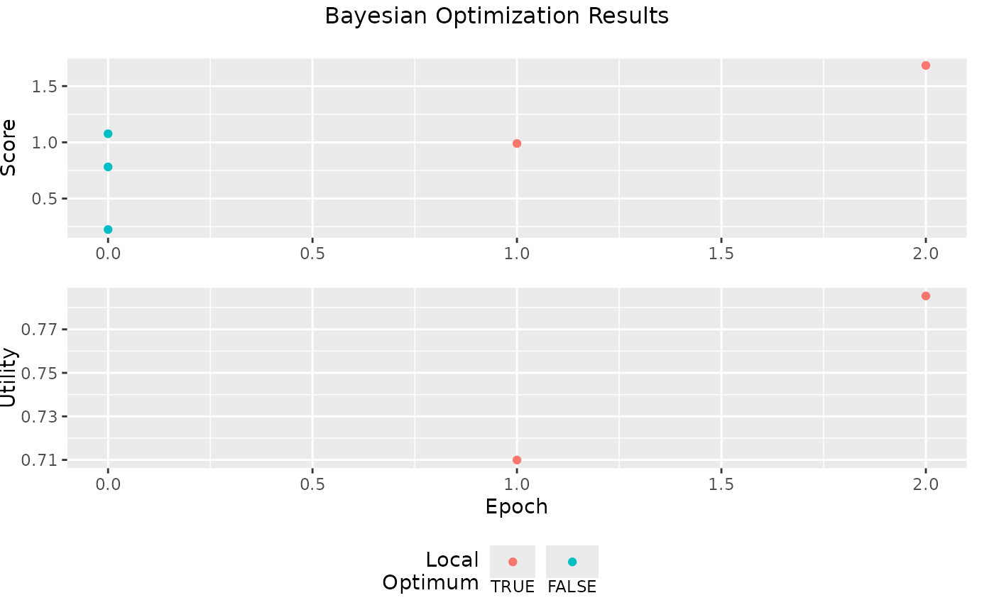
Returns 2 stacked plots - the top shows the results from FUN at each iteration. The bottom shows the utility from each point before the search took place.

Usage

# S3 method for class 'bayesOpt'
plot(x, ...)

Arguments

x

An object of class bayesOpt

...

Passed to patchwork::plot_layout(), overriding the defaults ncol = 1 and guides = "collect".

Value

A patchwork object, returned invisibly after printing.

Examples

scoringFunction <- function(x) {
  a <- exp(-(2-x)^2)*1.5
  b <- exp(-(4-x)^2)*2
  c <- exp(-(6-x)^2)*1
  return(list(Score = a+b+c))
}

bounds <- list(x = c(0,8))

Results <- bayesOpt(
    FUN = scoringFunction
  , bounds = bounds
  , initPoints = 3
  , iters.n = 2
  , gsPoints = 10
)
#> 
#> Running initial scoring function 3 times in 1 thread(s)...  0.535 seconds
#> 
#> Starting Epoch 1 
#>   1) Fitting Gaussian Process...
#>   2) Running local optimum search...        0.06 seconds
#>   3) Running FUN 1 times in 1 thread(s)...  0.188 seconds
#> 
#> Starting Epoch 2 
#>   1) Fitting Gaussian Process...
#>   2) Running local optimum search...        0.083 seconds
#>   3) Running FUN 1 times in 1 thread(s)...  0.185 seconds
# This plot will also show in real time with parameter plotProgress = TRUE in bayesOpt()
plot(Results)